The time-dependent Schrödinger equation and stationary states

The Schrödinger equation is the law of motion of quantum mechanics. Given the wave function at one moment, it determines the wave function at every later moment, as Newton's second law determines a classical trajectory from initial position and velocity. Erwin Schrödinger, a 38-year-old professor in Zurich, found it at the end of 1925 and published it in four papers during 1926, solving the hydrogen atom in the first. This lesson studies the equation itself: why it has the form it does, how separation of variables reduces it to an eigenvalue problem for the energy, what is special about the resulting stationary states, and how every other solution is built from them. That last idea, expanding a state in energy eigenstates and letting each term rotate in phase at its own frequency, is the single most used technique in the course.

The equation

For a particle of mass \(m\) in a potential \(V(x)\), the time-dependent Schrödinger equation is

The operator \(\hat H\) is the Hamiltonian, the energy operator, built from the classical energy \(p^2/2m + V\) by the substitution \(p \to -i\hbar\,\partial_x\) of lesson 2. The equation cannot be derived from classical physics; it is a postulate. But it can be motivated. A free particle with momentum \(p = \hbar k\) and energy \(E = \hbar\omega = p^2/2m\) should be a plane wave \(e^{i(kx - \omega t)}\). The time derivative brings down \(-i\omega\) and the second space derivative brings down \(-k^2\), so the plane wave satisfies \(i\hbar\,\partial_t\Psi = -(\hbar^2/2m)\partial_x^2\Psi\) exactly when \(\hbar\omega = \hbar^2k^2/2m\). The potential is then added so that the equation expresses energy conservation, \(E = p^2/2m + V\), term by term.

Three features of the equation shape everything that follows. It is first order in time, so the wave function at one instant is enough to determine the future, unlike the classical wave equation, which also needs the initial rate of change. It is linear, so sums of solutions are solutions, which is the mathematical home of superposition. And it contains \(i\) explicitly, so its solutions are necessarily complex; a real wave function at \(t = 0\) acquires an imaginary part at once.

Separation of variables

When \(V\) does not depend on time, try a product solution \(\Psi(x, t) = \psi(x)\,\varphi(t)\). Substituting and dividing by \(\psi\varphi\) gives

The left side depends only on \(t\) and the right only on \(x\). They can be equal for all \(x\) and \(t\) only if both equal the same constant, which we call \(E\). The time equation \(i\hbar\,d\varphi/dt = E\varphi\) has the solution \(\varphi = e^{-iEt/\hbar}\), and the space equation becomes the time-independent Schrödinger equation

This is an eigenvalue equation: \(\psi\) is an eigenfunction of the Hamiltonian and \(E\) is its eigenvalue. For a bound particle, solutions that can be normalized exist only for particular values of \(E\), the allowed energies \(E_1, E_2, E_3, \ldots\), with eigenfunctions \(\psi_1, \psi_2, \psi_3, \ldots\). Finding them is what is meant by solving a quantum system, and lessons 4 to 7 and 12 do it for the standard potentials.

Why the separable solutions matter

Separable solutions are special, but three properties make them central.

First, they are stationary. The probability density \(|\Psi|^2 = |\psi|^2\,|e^{-iEt/\hbar}|^2 = |\psi|^2\) does not depend on time, and neither does any expectation value \(\langle Q\rangle = \int\psi^{*}\hat Q\psi\,dx\), because the phase factors \(e^{\pm iEt/\hbar}\) cancel. Nothing observable changes. In particular \(\langle x\rangle\) is constant, so \(\langle p\rangle = 0\) for every stationary state. An electron in a stationary state of an atom does not orbit in any observable sense, which is why it does not radiate, resolving the classical collapse of the atom that PHYS-271 described.

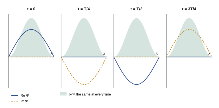
Second, they have definite energy. Applying \(\hat H\) twice gives \(\hat H^2\psi = E^2\psi\), so \(\langle H^2\rangle = E^2 = \langle H\rangle^2\) and the spread \(\sigma_H = \sqrt{\langle H^2\rangle - \langle H\rangle^2}\) is zero. Every measurement of the energy of a particle in the state \(\psi_n\) returns \(E_n\), with certainty.

Third, and most important, every solution of the time-dependent equation is a superposition of separable ones. For the potentials of this course, the eigenfunctions form a complete set, meaning that any reasonable initial wave function can be expanded as \(\Psi(x, 0) = \sum_n c_n\psi_n(x)\). Then, because the equation is linear and each term evolves with its own phase,

This is the general solution. To find it, expand the initial state in eigenfunctions, attach a phase \(e^{-iE_nt/\hbar}\) to each coefficient, and add up. When the eigenfunctions are orthonormal, \(\int\psi_m^{*}\psi_n\,dx = \delta_{mn}\), as they will be (lesson 8 proves it for any Hermitian operator), the coefficients are found by projection, \(c_n = \int\psi_n^{*}\,\Psi(x, 0)\,dx\), exactly as the components of a vector are found by dot products with basis vectors.

The coefficients have a physical meaning. Normalization of \(\Psi\) becomes \(\sum|c_n|^2 = 1\), and the expectation value of the energy is \(\langle H\rangle = \sum|c_n|^2E_n\). Both are constant in time, because the phases cancel in \(|c_ne^{-iE_nt/\hbar}|^2\). The number \(|c_n|^2\) is the probability that a measurement of the energy gives \(E_n\), the general Born rule of lesson 9. A superposition of states with different energies is not stationary: its density contains cross terms with time dependence \(\cos[(E_m - E_n)t/\hbar]\), so it oscillates at the Bohr frequencies \((E_m - E_n)/h\). Those are exactly the frequencies of light an atom emits or absorbs in a transition between the two levels.

General facts about the energies

Several properties of the time-independent equation hold for any potential and save effort later.

The separation constant \(E\) must be real for normalizable solutions. If \(E = E_0 + i\Gamma\), then \(|\Psi|^2 = |\psi|^2e^{2\Gamma t/\hbar}\), which grows or decays in time, contradicting conservation of probability (lesson 2). Complex energies do appear, but as descriptions of decaying states that are not normalizable, a topic for PHYS-373.

The energy must exceed the minimum of the potential. Rearranging the equation gives \(\psi'' = (2m/\hbar^2)(V - E)\psi\). If \(E < V\) everywhere, then \(\psi''\) always has the same sign as \(\psi\), so the function curves away from the axis and grows without bound in at least one direction. No normalizable solution exists. A bound state with \(E\) below the bottom of the well is impossible.

Eigenfunctions can be taken real. The equation has real coefficients, so if \(\psi\) is a solution, so are \(\psi^{*}\), \(\mathrm{Re}\,\psi\) and \(\mathrm{Im}\,\psi\), all with the same energy. For a bound state in one dimension, where each energy has only one independent eigenfunction, \(\psi\) is a real function times a constant phase.

Symmetric potentials give eigenfunctions of definite parity. If \(V(-x) = V(x)\), then \(\psi(-x)\) is a solution whenever \(\psi(x)\) is, so the eigenfunctions can be chosen even or odd. This halves the work for wells symmetric about the origin, as lesson 7 shows.

In one dimension, bound states are nondegenerate: no two independent bound eigenfunctions share an energy. If \(\psi_1\) and \(\psi_2\) both solve the equation with energy \(E\), then \(\psi_1\psi_2'' - \psi_2\psi_1'' = 0\), so the Wronskian \(\psi_1\psi_2' - \psi_2\psi_1'\) is constant; it vanishes at infinity, where both functions do, so it is zero everywhere and \(\psi_2\) is a multiple of \(\psi_1\). The ground state has no nodes, and the \(n\)th state has \(n - 1\), a pattern every example will display.

Solving the time-dependent equation directly

The eigenfunction expansion is exact when the eigenfunctions are known. When they are not, the time-dependent equation can be integrated numerically. The program below does both for a particle in a box of width \(L\), starting in an equal superposition of the two lowest states. It evolves the state once by the expansion formula and once with the Crank–Nicolson method, which replaces \(e^{-i\hat H\Delta t/\hbar}\) by \((1 + i\hat H\Delta t/2\hbar)^{-1}(1 - i\hat H\Delta t/2\hbar)\). That approximation is unitary, so it conserves probability exactly at every step, and each step needs only a tridiagonal linear solve. The two methods agree, the norm stays at one, \(\langle H\rangle\) stays constant, and \(\langle x\rangle\) oscillates with the period \(h/(E_2 - E_1)\).

import cmath, math
hbar = m = 1.0; Lbox = 1.0
N = 200; dx = Lbox / (N + 1)
xs = [(j + 1) * dx for j in range(N)]                 # interior grid points
E = lambda n: (n * math.pi * hbar) ** 2 / (2 * m * Lbox ** 2)
phi = lambda n, x: math.sqrt(2 / Lbox) * math.sin(n * math.pi * x / Lbox)
psi0 = [(phi(1, x) + phi(2, x)) / math.sqrt(2) for x in xs]
T = 2 * math.pi * hbar / (E(2) - E(1))                # period of the beat
def exact(t):
    return [(phi(1, x) * cmath.exp(-1j * E(1) * t) + phi(2, x) * cmath.exp(-1j * E(2) * t)) / math.sqrt(2) for x in xs]
# Crank-Nicolson: (1 + i dt H / 2) psi_new = (1 - i dt H / 2) psi_old, H tridiagonal
steps = 400; dt = T / steps
off = -hbar ** 2 / (2 * m * dx ** 2); diag = -2 * off
a = 1j * dt / (2 * hbar)
def cn_step(p):
    rhs = [(1 - a * diag) * p[j] - a * off * ((p[j - 1] if j else 0) + (p[j + 1] if j < N - 1 else 0)) for j in range(N)]
    c = [0j] * N; d = [0j] * N                         # Thomas algorithm
    bm, om = 1 + a * diag, a * off
    c[0] = om / bm; d[0] = rhs[0] / bm
    for j in range(1, N):
        den = bm - om * c[j - 1]
        c[j] = om / den; d[j] = (rhs[j] - om * d[j - 1]) / den
    out = [0j] * N; out[-1] = d[-1]
    for j in range(N - 2, -1, -1): out[j] = d[j] - c[j] * out[j + 1]
    return out
def stats(p):
    norm = sum(abs(v) ** 2 for v in p) * dx
    xm = sum(x * abs(v) ** 2 for x, v in zip(xs, p)) * dx
    Hp = [diag * p[j] + off * ((p[j - 1] if j else 0) + (p[j + 1] if j < N - 1 else 0)) for j in range(N)]
    H = sum((p[j].conjugate() * Hp[j]).real for j in range(N)) * dx
    return norm, xm, H
p = [complex(v) for v in psi0]
print(f"E1 = {E(1):.4f}, E2 = {E(2):.4f}, beat period T = {T:.4f}  (units hbar = m = L = 1)")
print(" t/T   norm(CN)   <x> CN    <x> exact   <H> CN   max |CN - exact|")
for k in range(steps + 1):
    if k % 100 == 0:
        t = k * dt; ex = exact(t)
        n_, xm, H = stats(p); _, xe, _ = stats(ex)
        err = max(abs(u - v) for u, v in zip(p, ex))
        print(f"{t / T:4.2f}  {n_:.6f}  {xm:.5f}   {xe:.5f}    {H:.3f}    {err:.1e}")
    p = cn_step(p)

E1 = 4.9348, E2 = 19.7392, beat period T = 0.4244  (units hbar = m = L = 1)
 t/T   norm(CN)   <x> CN    <x> exact   <H> CN   max |CN - exact|
0.00  1.000000  0.31987   0.31987    12.336    0.0e+00
0.25  1.000000  0.49996   0.50000    12.336    2.5e-04
0.50  1.000000  0.68013   0.68013    12.336    5.1e-04
0.75  1.000000  0.50013   0.50000    12.336    7.4e-04
1.00  1.000000  0.31987   0.31987    12.336    1.0e-03

The mean position swings from the left half of the box to the right and back once per beat period, while the norm stays at one to the printed precision. The small differences between the two methods come from the finite grid, which slightly lowers the discretized energies, and from the Crank–Nicolson time step; both shrink as the grid and step are refined. The value of \(\langle H\rangle\) lies between \(E_1\) and \(E_2\), equal to their average because the coefficients have equal magnitude.

Phases, clocks and spectra

The phase factor \(e^{-iEt/\hbar}\) of a stationary state is unobservable on its own, since an overall phase never matters. But relative phases between energy components are the clock hands of quantum mechanics. Every observable change in a quantum system is a beat between two or more energies, at frequency \(\Delta E/h\). The cesium atomic clock that defines the second counts \(9\,192\,631\,770\) beats per second between two hyperfine levels of the cesium-133 ground state; the optical clocks being developed at national laboratories, including NRC in Ottawa and NIST in Boulder, use beats near \(10^{15}\) Hz between levels of ions or atoms. The precision of such clocks, better than one part in \(10^{18}\), rests on the simple statement that a superposition of two stationary states oscillates at exactly the difference of their energies divided by \(h\).