Degenerate Fermi gases: electrons in metals and white dwarfs

When a gas of fermions is so dense, or so cold, that \(n\lambda^3 \gg 1\), the exclusion principle dominates everything. The particles fill the lowest available orbitals one at a time, up to an energy far above \(kT\), and the gas behaves very differently from a classical one: it has a large energy and pressure even at absolute zero, a heat capacity much smaller than equipartition predicts, and a strange relation between mass and size when it is held together by gravity. Such a gas is called degenerate. This lesson works out the theory of the degenerate Fermi gas and applies it to its two most important examples: the conduction electrons in a metal, and the matter in white dwarf stars, which led Subrahmanyan Chandrasekhar to the maximum mass that bears his name.

The Fermi sea at absolute zero

At \(T = 0\), the Fermi–Dirac distribution is a step: every orbital with \(\varepsilon < \mu\) holds exactly one fermion and every orbital above is empty. The chemical potential at zero temperature is called the Fermi energy \(E_F\). In momentum space the occupied orbitals fill a sphere of radius \(p_F = \sqrt{2mE_F}\), the Fermi sphere. Counting the orbitals inside it, with spin degeneracy 2 for electrons,

The Fermi energy depends only on the density. The total energy follows from integrating \(\varepsilon\,g(\varepsilon)\) up to \(E_F\) with \(g \propto \sqrt\varepsilon\), which gives \(U = \frac35 NE_F\): the average fermion has three fifths of the Fermi energy, even at absolute zero. Because \(E_F \propto V^{-2/3}\), the energy depends on volume, and the gas exerts a degeneracy pressure

This pressure has nothing to do with temperature. It arises because squeezing the gas raises the energies of all occupied orbitals, and it is the reason matter is hard to compress. The first part of the program evaluates these quantities for three metals with the free-electron densities of their conduction electrons. Copper has \(E_F = 7.0\) eV, which corresponds to a Fermi temperature \(T_F = E_F/k\) of 82,000 K, and a Fermi velocity of \(1.6 \times 10^6\) m/s, about one two-hundredth of the speed of light. At room temperature \(T/T_F\) is about 0.004, so a metal at 300 K is, as far as its electrons are concerned, extremely cold.

The degeneracy pressure of copper's electrons is 38 GPa, about 400,000 atmospheres, balanced in a real metal by the attraction of the electrons to the positive ions. A rough estimate of the compressibility follows: the bulk modulus of the electron gas, \(B = -V\,\partial P/\partial V = \frac53 P\), is 64 GPa for copper, within a factor of about two of the measured value. For the alkali metals, where the free-electron model works best, the agreement is closer.

Finite temperature and the Sommerfeld expansion

At a small nonzero temperature, the step in the occupancy is rounded over an energy range of a few \(kT\) around \(\mu\). Only electrons within about \(kT\) of the Fermi energy can be thermally excited; electrons deep in the Fermi sea have no empty states nearby to move into. The number of excitable electrons is therefore about \(g(E_F)kT\), a fraction of order \(kT/E_F\) of the total, and each gains energy of order \(kT\). The thermal energy is of order \(N(kT)^2/E_F\), and the heat capacity is linear in \(T\) and smaller than the classical \(\frac32 Nk\) by a factor of order \(T/T_F\).

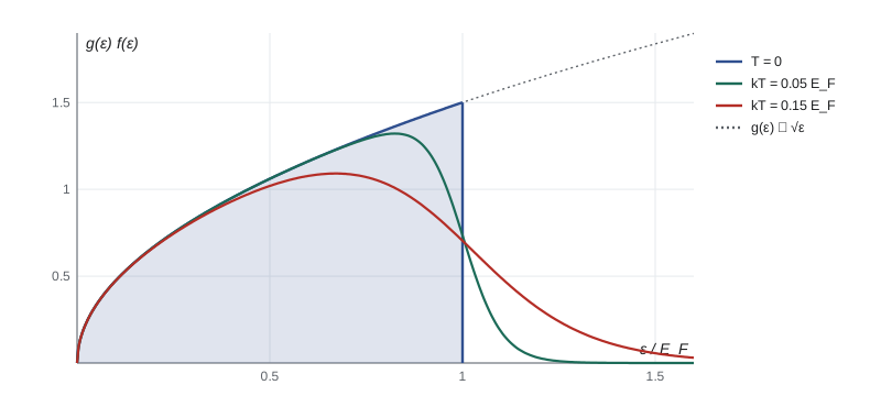
Arnold Sommerfeld made this precise in 1927 and 1928, with an expansion of integrals of the form \(\int\phi(\varepsilon)f(\varepsilon)d\varepsilon\) in powers of \(kT/\mu\). The derivative of the Fermi function is sharply peaked at \(\mu\), with width \(kT\), so expanding \(\phi\) about \(\mu\) and integrating term by term gives

The \(\pi^2/6\) comes from the integral \(\int x^2e^x/(e^x + 1)^2dx = \pi^2/3\). Applying the formula to \(N\) and \(U\) gives the chemical potential and heat capacity to leading order:

The second part of the program checks both formulas by integrating the Fermi–Dirac distribution numerically, finding \(\mu\) by bisection on the particle number and differentiating the energy. At \(kT = 0.01E_F\) the numerical heat capacity and the Sommerfeld formula agree to all printed digits.

import math
hbar = 1.054571817e-34; h = 2 * math.pi * hbar; me = 9.1093837e-31; k = 1.380649e-23
eV = 1.602176634e-19; c = 2.99792458e8; G = 6.6743e-11; u = 1.66053907e-27; Msun = 1.98892e30; NA = 6.02214076e23

# 1. Free-electron Fermi energies
print("Free-electron model")
for metal, n in (('Na', 2.65e28), ('Cu', 8.47e28), ('Al', 18.1e28)):
    EF = hbar ** 2 / (2 * me) * (3 * math.pi ** 2 * n) ** (2 / 3)
    vF = math.sqrt(2 * EF / me)
    P = 0.4 * n * EF
    gamma = math.pi ** 2 * NA * k ** 2 / (2 * EF)   # per mole of electrons
    print(f"  {metal}: E_F = {EF / eV:5.2f} eV, T_F = {EF / k:8.0f} K, v_F = {vF:.2e} m/s, "
          f"degeneracy pressure {P / 1e9:5.1f} GPa, gamma = {gamma * 1000:.3f} mJ/(mol K^2)")

# 2. Sommerfeld check: heat capacity of the electron gas by direct integration (units E_F = 1)
def energy(t):
    """Total energy per electron at kT = t, with mu fixed by the particle number."""
    g = lambda e: 1.5 * math.sqrt(e)                 # density of states, normalized to 1 below E_F
    def count(mu):
        return sum(g(e) / (math.exp((e - mu) / t) + 1) * de for e in grid)
    lo, hi = 0.9, 1.1
    for _ in range(50):
        mid = (lo + hi) / 2
        if count(mid) < 1: lo = mid
        else: hi = mid
    mu = (lo + hi) / 2
    return sum(e * g(e) / (math.exp((e - mu) / t) + 1) * de for e in grid), mu
de = 2e-4
grid = [de * (i + 0.5) for i in range(int(1.6 / de))]
for t in (0.01, 0.02):
    (E1, mu1), (E2, mu2) = energy(t * 0.99), energy(t * 1.01)
    C = (E2 - E1) / (0.02 * t)                       # dE/d(kT): C/(N k)
    print(f"  kT/E_F = {t}: C/(Nk) numerical {C:.4f}, Sommerfeld (pi^2/2) kT/E_F = {math.pi ** 2 / 2 * t:.4f}, "
          f"mu/E_F = {mu1:.5f} (expect 1 - (pi^2/12)(kT/E_F)^2 = {1 - math.pi ** 2 / 12 * (t * 0.99) ** 2:.5f})")

Free-electron model
  Na: E_F =  3.24 eV, T_F =    37612 K, v_F = 1.07e+06 m/s, degeneracy pressure   5.5 GPa, gamma = 1.091 mJ/(mol K^2)
  Cu: E_F =  7.03 eV, T_F =    81612 K, v_F = 1.57e+06 m/s, degeneracy pressure  38.2 GPa, gamma = 0.503 mJ/(mol K^2)
  Al: E_F = 11.67 eV, T_F =   135399 K, v_F = 2.03e+06 m/s, degeneracy pressure 135.3 GPa, gamma = 0.303 mJ/(mol K^2)
  kT/E_F = 0.01: C/(Nk) numerical 0.0493, Sommerfeld (pi^2/2) kT/E_F = 0.0493, mu/E_F = 0.99992 (expect 1 - (pi^2/12)(kT/E_F)^2 = 0.99992)
  kT/E_F = 0.02: C/(Nk) numerical 0.0986, Sommerfeld (pi^2/2) kT/E_F = 0.0987, mu/E_F = 0.99968 (expect 1 - (pi^2/12)(kT/E_F)^2 = 0.99968)

The heat capacity of metals

The electronic heat capacity explained a long-standing puzzle. Paul Drude's classical model of 1900 treated conduction electrons as a gas, which successfully explained electrical and thermal conductivity but predicted an extra \(\frac32 R\) per mole of electrons in the heat capacity. No such contribution was seen: metals obey Dulong and Petit just like insulators. Sommerfeld's theory shows why: at room temperature the electronic term is less than one hundredth of the classical value. It is not zero, however. At low temperature, the lattice heat capacity falls as \(T^3\) (lesson 10) while the electronic one falls only as \(T\), so below a few kelvin the electrons dominate. Measured heat capacities of metals fit the form \(C = \gamma T + \beta T^3\), and plotting \(C/T\) against \(T^2\) gives a straight line whose intercept is \(\gamma\).

The free-electron model predicts \(\gamma = \pi^2N_Ak^2/2E_F\) per mole of conduction electrons: 0.50 mJ/(mol K²) for copper, as the program shows. The measured value is about 0.69 mJ/(mol K²). The ratio, about 1.4, is a measure of how the electrons' interactions with the lattice and with each other increase their effective mass. In some compounds of cerium and uranium, called heavy-fermion materials, \(\gamma\) is hundreds of times the free-electron value. The same \(g(E_F)\) controls the Pauli paramagnetism of metals, which is small and nearly independent of temperature, again because only electrons near the Fermi energy can respond.

White dwarfs

A star like the Sun ends its life by shedding its outer layers and leaving behind a hot, dense core about the size of Earth: a white dwarf. Sirius B, the companion of the brightest star in the night sky, is one, with about the mass of the Sun in a body roughly the size of the Earth. The density is around a tonne per cubic centimetre. No nuclear fusion supports it against gravity. In 1926 Ralph Fowler, applying the brand-new Fermi–Dirac statistics, showed that the electrons in such a star are a degenerate gas whose pressure holds it up even when it has cooled. White dwarfs were the first astronomical objects explained by quantum statistics.

A simple estimate gives the mass–radius relation. For a star of mass \(M\) and radius \(R\), made of carbon and oxygen with \(\mu_e = 2\) nucleons per electron, the electron density is \(n \propto M/R^3\), so the degeneracy energy per electron is \(E_F \propto n^{2/3} \propto M^{2/3}/R^2\) and the total kinetic energy is of order \(M\cdot M^{2/3}/R^2\). The gravitational energy is of order \(-GM^2/R\). Minimizing the sum over \(R\) gives

Heavier white dwarfs are smaller. This is opposite to ordinary matter, and it leads to a catastrophe. As \(M\) grows, the star shrinks, the density rises, and the Fermi momentum of the electrons becomes comparable to \(m_ec\). The electrons become relativistic, their energy becomes \(cp\) instead of \(p^2/2m\), and the degeneracy energy per electron scales as \(n^{1/3} \propto M^{1/3}/R\) instead. Now both the kinetic and the gravitational energies scale as \(1/R\), and shrinking no longer helps: if the mass exceeds a critical value, gravity wins at every radius.

Chandrasekhar found the critical mass in 1930 and 1931, at the age of about 20. Working it out exactly requires solving hydrostatic equilibrium, \(dP/dr = -Gm(r)\rho/r^2\), with the exact pressure of a degenerate electron gas of any momentum. The program below does this with a fourth-order Runge–Kutta integration from the centre outward, for a range of central densities, using the variable \(x^2\) where \(x = p_F/m_ec\) so the integration behaves well at the surface.

import math
hbar = 1.054571817e-34; h = 2 * math.pi * hbar; me = 9.1093837e-31; c = 2.99792458e8
G = 6.6743e-11; u = 1.66053907e-27; Msun = 1.98892e30; Rearth = 6.371e6
mu_e = 2.0                                   # nucleons per electron (helium, carbon, oxygen)
lam = hbar / (me * c)                        # reduced Compton wavelength
K = math.pi * me ** 4 * c ** 5 / (3 * h ** 3)
rho_of = lambda x: mu_e * u * x ** 3 / (3 * math.pi ** 2 * lam ** 3)   # x = p_F/(m_e c)
dPdx = lambda x: K * 8 * x ** 4 / math.sqrt(1 + x * x)                # from the exact degenerate P(x)

def star(xc):
    """Integrate hydrostatic equilibrium outward; variables s = x^2 and enclosed mass m."""
    r = 1.0
    s, m = xc * xc, 4 / 3 * math.pi * r ** 3 * rho_of(xc)
    # scale the step to the expected radius
    dr = 2e7 / max(xc, 0.3) / 2000
    def deriv(r, s, m):
        x = math.sqrt(max(s, 1e-30))
        dxdr = -G * m * rho_of(x) / (r * r * dPdx(x))
        return 2 * x * dxdr, 4 * math.pi * r * r * rho_of(x)
    while s > 0:
        k1 = deriv(r, s, m); k2 = deriv(r + dr / 2, s + dr / 2 * k1[0], m + dr / 2 * k1[1])
        k3 = deriv(r + dr / 2, s + dr / 2 * k2[0], m + dr / 2 * k2[1]); k4 = deriv(r + dr, s + dr * k3[0], m + dr * k3[1])
        s_new = s + dr / 6 * (k1[0] + 2 * k2[0] + 2 * k3[0] + k4[0])
        m_new = m + dr / 6 * (k1[1] + 2 * k2[1] + 2 * k3[1] + k4[1])
        if s_new <= 0:
            r += dr * s / (s - s_new); break        # linear interpolation to the surface
        r, s, m = r + dr, s_new, m_new
    return m / Msun, r

print("Degenerate electron stars (mu_e = 2): central x = p_F/(m_e c), mass, radius")
for xc in (0.3, 1.0, 3.0, 10.0, 30.0, 100.0):
    M, R = star(xc)
    print(f"  x_c = {xc:6.1f}: central density {rho_of(xc):.2e} kg/m^3, M = {M:.4f} solar masses, "
          f"R = {R / 1000:7.0f} km ({R / Rearth:.3f} Earth radii)")
M_ch = 5.836 / mu_e ** 2
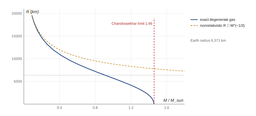
print(f"Chandrasekhar's limiting mass 5.836/mu_e^2 = {M_ch:.3f} solar masses")

Degenerate electron stars (mu_e = 2): central x = p_F/(m_e c), mass, radius
  x_c =    0.3: central density 5.26e+07 kg/m^3, M = 0.1098 solar masses, R =   18255 km (2.865 Earth radii)
  x_c =    1.0: central density 1.95e+09 kg/m^3, M = 0.5101 solar masses, R =    9704 km (1.523 Earth radii)
  x_c =    3.0: central density 5.26e+10 kg/m^3, M = 1.0955 solar masses, R =    4998 km (0.785 Earth radii)
  x_c =   10.0: central density 1.95e+12 kg/m^3, M = 1.3943 solar masses, R =    2073 km (0.325 Earth radii)
  x_c =   30.0: central density 5.26e+13 kg/m^3, M = 1.4476 solar masses, R =     806 km (0.127 Earth radii)
  x_c =  100.0: central density 1.95e+15 kg/m^3, M = 1.4551 solar masses, R =     259 km (0.041 Earth radii)
Chandrasekhar's limiting mass 5.836/mu_e^2 = 1.459 solar masses

Low-density models follow the nonrelativistic \(R \propto M^{-1/3}\). As the central density rises the mass approaches a limit of 1.46 solar masses while the radius shrinks toward zero. Chandrasekhar's analytic value for \(\mu_e = 2\) is \(5.836/\mu_e^2 = 1.459\) solar masses, matched by the integration. A model of 1.1 solar masses has a radius of about 5,000 km, smaller than the Earth.

The Chandrasekhar limit has enormous consequences. A white dwarf that gains mass from a companion until it approaches the limit ignites carbon fusion and explodes as a type Ia supernova; because these explosions all happen near the same mass, they have similar peak brightness, which made them the standard candles that revealed the accelerating expansion of the universe in 1998. A stellar core above the limit cannot be supported by electrons at all; it collapses until neutrons, also fermions, become degenerate, forming a neutron star about 20 km across, or, if heavier still, a black hole. Chandrasekhar's result was resisted for years, notably by Arthur Eddington, and he received the Nobel Prize in Physics in 1983.