The grand canonical ensemble and chemical potential

Temperature governs the flow of energy; chemical potential governs the flow of particles. Molecules evaporate from a liquid into its vapour, dissolve into a solution, bind to a protein, react to form new species, or diffuse from one region of a container to another, always moving from high chemical potential to low. This lesson develops the chemical potential as a physical quantity, calculates it for an ideal gas, and then builds the third standard ensemble, in which a system exchanges both energy and particles with a reservoir. The grand canonical ensemble is the natural home of binding and adsorption problems, and it is the essential tool for the quantum gases of the next three lessons, because it lets each single-particle state be treated as a separate system.

What chemical potential means

Lesson 3 defined \(\mu = -T(\partial S/\partial N)_{U,V}\) and showed that two systems exchanging particles come to equilibrium when their chemical potentials are equal. Equivalent forms follow from the thermodynamic identity: \(\mu = (\partial U/\partial N)_{S,V} = (\partial F/\partial N)_{T,V} = (\partial G/\partial N)_{T,P}\). The last form says that for a single substance \(\mu\) is the Gibbs free energy per particle, \(G = N\mu\). Chemical potential is an energy, measured in joules or electronvolts per particle (or joules per mole), and like any energy its zero is a matter of convention; only differences between chemical potentials are physical.

Particles flow from high \(\mu\) to low \(\mu\) because the total entropy then rises: removing a particle from a region of high \(\mu\) raises that region's entropy by \(\mu/T\), and adding it to a region of low \(\mu\) lowers that region's entropy by less. Equality of chemical potential is the condition for phase equilibrium (ice and water coexist at 0 °C at 1 atm because their chemical potentials are equal there), for diffusive equilibrium between regions, and, as lesson 12 shows, for chemical equilibrium between reacting species.

The chemical potential of an ideal gas

For an ideal gas, lesson 6 gave \(F = -NkT[\ln(VZ_{\text{int}}/N\lambda^3) + 1]\). Differentiating with respect to \(N\),

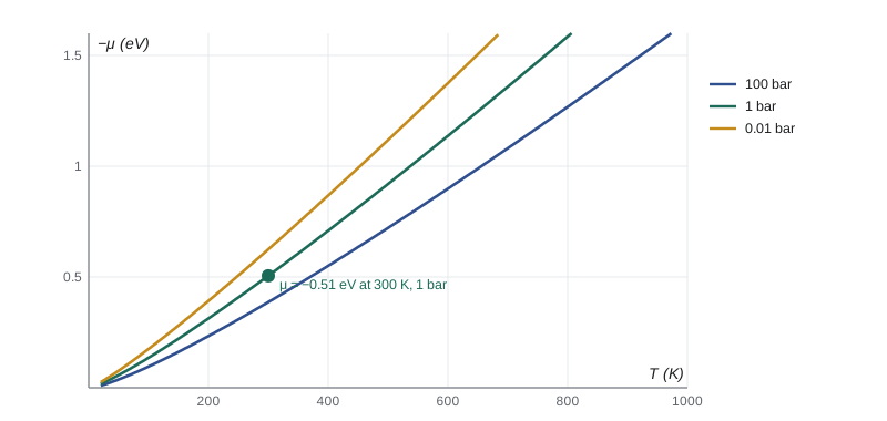
For a dilute gas, \(n\lambda^3\) is very small, so the logarithm is large and negative: \(\mu\) is negative and of order several \(kT\). The chemical potential rises logarithmically with density: multiplying the density by 10 adds \(kT\ln 10\), which is 0.06 eV at room temperature. And it falls as the temperature rises, because \(\lambda\) shrinks and more internal states become available. The program computes \(\mu\) for nitrogen at 300 K and 1 bar: \(-0.40\) eV from translation alone and \(-0.51\) eV once rotation is included. The quantity \(1/\lambda^3\), called the quantum concentration \(n_Q\), sets the scale: the gas is classical when \(n \ll n_Q\), which lesson 8 explores.

Chemical potential in an external field

If particles also have potential energy \(V(\mathbf r)\), for example in gravity, their chemical potential gains a term \(V\): \(\mu = kT\ln(n\lambda^3/Z_{\text{int}}) + V(\mathbf r)\). In equilibrium \(\mu\) must be the same everywhere, otherwise particles would flow. For gravity, \(V = mgz\), so at constant temperature

This is the barometric formula, which PHYS-261 derived from the Boltzmann distribution, now obtained from the balance of chemical potential. The scale height \(kT/mg\) is 7.6 km for nitrogen at 250 K. The same reasoning describes ions in an electric potential, where it gives the Boltzmann distribution of charge in an electrolyte near an electrode, and electrons in a semiconductor, where the equality of the chemical potential (called the Fermi level there) across a junction explains the built-in voltage of a diode.

The grand canonical ensemble

Now let a system exchange both energy and particles with a large reservoir at temperature \(T\) and chemical potential \(\mu\). Repeating the argument of lesson 4, the probability of a system microstate \(s\) with energy \(E_s\) and particle number \(N_s\) is proportional to the reservoir's multiplicity, and expanding the reservoir's entropy to first order in both energy and particle number gives

Therefore the probability is proportional to the Gibbs factor,

where the grand partition function \(\mathcal Z\) sums over all states with all particle numbers. Averages follow by differentiation, as before. The mean particle number is \(\bar N = kT\,\partial\ln\mathcal Z/\partial\mu\), and the grand potential \(\Phi = -kT\ln\mathcal Z = U - TS - \mu N\) plays the role that \(F\) played in the canonical ensemble. For a homogeneous system, \(\Phi = -PV\). The fluctuation in particle number obeys

another fluctuation–dissipation relation. For an ideal gas, \(\bar N = (V/\lambda^3)e^{\mu/kT}\), so \(\partial\bar N/\partial\mu = \bar N/kT\) and \(\sigma_N^2 = \bar N\): the number of molecules in an open region follows a Poisson distribution. The program checks this by randomly placing 1,000 particles in a box and counting how many land in a subvolume holding one twentieth of the space. The variance comes out close to the mean, slightly less because the box itself is finite (a binomial distribution, with variance \(\bar N(1 - p)\)). Near a liquid–gas critical point, \(\partial\bar N/\partial\mu\) becomes enormous, the density fluctuations grow to the scale of the wavelength of light, and the fluid turns milky, an effect called critical opalescence.

import math, random
k = 1.380649e-23; h = 6.62607015e-34; u = 1.66053907e-27; eV = 1.602176634e-19
rnd = random.Random(361)

def mu_ideal(m, T, n, zint=1.0):
    """Chemical potential (J) of an ideal gas with internal partition function zint."""
    lam = h / math.sqrt(2 * math.pi * m * k * T)
    return -k * T * math.log(zint / (n * lam ** 3))

# 1. Chemical potential of nitrogen at 300 K and 1 bar, translation only and with rotation
T, P = 300.0, 1.0e5
n = P / (k * T)
m = 28.014 * u
zrot = T / (2 * 2.88)                    # theta_rot = 2.88 K, symmetry number 2
print(f"N2 at 300 K, 1 bar: n = {n:.3e} per m^3")
print(f"  mu (translation only)       = {mu_ideal(m, T, n) / eV:+.3f} eV")
print(f"  mu (translation + rotation) = {mu_ideal(m, T, n, zrot) / eV:+.3f} eV")
for f in (10, 0.1):
    print(f"  at {f} times the density, mu changes by kT ln {f} = {k * T * math.log(f) / eV:+.4f} eV")

# 2. Barometric formula from equal chemical potential at every height
g, T = 9.81, 250.0
H = k * T / (m * g)
print(f"\nIsothermal atmosphere at 250 K: scale height kT/mg = {H / 1000:.2f} km for N2")

# 3. Number fluctuations in an open subvolume (grand canonical): variance = mean for an ideal gas
M, p, trials = 1000, 0.05, 3000      # particles in the big box, subvolume fraction
counts = []
for _ in range(trials):
    counts.append(sum(1 for _ in range(M) if rnd.random() < p))
mean = sum(counts) / trials
var = sum((c - mean) ** 2 for c in counts) / (trials - 1)
print(f"\nSubvolume holding {p} of a {M}-particle box: mean {mean:.2f}, variance {var:.2f}, "
      f"Poisson prediction {M * p:.2f} (finite box gives {M * p * (1 - p):.2f})")

# 4. A binding site in contact with oxygen gas (simplified Gibbs-factor model)
T = 310.0
P_O2 = 0.21 * 1.013e5
n = P_O2 / (k * T)
m = 31.998 * u
zint = (T / (2 * 2.08)) * 3              # rotation (theta 2.08 K, sigma 2) and spin triplet ground state
mu = mu_ideal(m, T, n, zint)
print(f"\nO2 at 310 K and 0.21 atm: mu = {mu / eV:+.3f} eV")
for eps in (-0.60, -0.65, -0.70, -0.75):
    x = math.exp(-(eps * eV - mu) / (k * T))        # Gibbs factor of the occupied state
    print(f"  binding energy {eps:+.2f} eV: occupied fraction {x / (1 + x):.3f}")

N2 at 300 K, 1 bar: n = 2.414e+25 per m^3
  mu (translation only)       = -0.403 eV
  mu (translation + rotation) = -0.506 eV
  at 10 times the density, mu changes by kT ln 10 = +0.0595 eV
  at 0.1 times the density, mu changes by kT ln 0.1 = -0.0595 eV

Isothermal atmosphere at 250 K: scale height kT/mg = 7.56 km for N2

Subvolume holding 0.05 of a 1000-particle box: mean 49.98, variance 47.04, Poisson prediction 50.00 (finite box gives 47.50)

O2 at 310 K and 0.21 atm: mu = -0.610 eV
  binding energy -0.60 eV: occupied fraction 0.405
  binding energy -0.65 eV: occupied fraction 0.816
  binding energy -0.70 eV: occupied fraction 0.966
  binding energy -0.75 eV: occupied fraction 0.995

Vapour pressure from equal chemical potentials

Equality of chemical potential predicts the vapour pressure of a solid in a few lines. Model the solid as atoms bound with energy \(-\Delta\) each, relative to a free atom at rest, and vibrating as Einstein oscillators. At temperatures well above the Einstein temperature, each atom in the solid contributes \(Z_{\text{sol}} = e^{\Delta/kT}(kT/\hbar\omega)^3\) to the partition function, and because the atoms sit on distinguishable lattice sites there is no \(1/N!\). The chemical potential of the solid is then \(\mu_{\text{sol}} = -kT\ln Z_{\text{sol}} = -\Delta - 3kT\ln(kT/\hbar\omega)\). Setting it equal to the chemical potential of the vapour, \(kT\ln(n\lambda^3)\), and solving for the pressure \(P = nkT\) gives

The exponential factor dominates. It reproduces the Clausius–Clapeyron behaviour of PHYS-261, with the binding energy per atom playing the role of the latent heat of sublimation, and the prefactor, which thermodynamics alone cannot supply, follows from the partition functions. Every vapour-pressure curve, from the frost on a Prairie window in winter to the evaporation of a metal filament, has this structure: an energy cost for leaving the condensed phase, weighed against the enormous number of translational states available in the gas.

A single binding site

The grand canonical ensemble is ideal for problems where one site can hold a particle or not. Consider a site on a protein or a surface that can be empty (energy 0) or occupied by one molecule (energy \(\varepsilon < 0\), the binding energy), in contact with a gas or solution that sets \(\mu\). Then

The site is half full when \(\varepsilon = \mu\), and the occupancy switches from nearly 0 to nearly 1 over a range of a few \(kT\) in \(\varepsilon - \mu\). The program applies this to oxygen in air at body temperature, where \(\mu = -0.61\) eV once rotation and the triplet ground state are included. A binding energy of \(-0.60\) eV gives an occupancy of 0.405; \(-0.65\) eV gives 0.82; \(-0.70\) eV gives 0.97. Small changes in binding energy produce large changes in occupancy. Real oxygen-binding proteins are more complicated, with internal partition functions for the bound state and cooperative binding among several sites, but this one-site model captures the switching behaviour. It also shows why carbon monoxide, which binds more strongly, is so dangerous even at low concentration: a competing molecule changes the grand partition function to \(1 + e^{-(\varepsilon_1 - \mu_1)/kT} + e^{-(\varepsilon_2 - \mu_2)/kT}\).

Fermi and Bose statistics in one line

The binding-site result already contains the Fermi–Dirac distribution. A single quantum state (an orbital) of energy \(\varepsilon\) that can hold at most one fermion is exactly a binding site, so its mean occupancy is \(1/(e^{(\varepsilon - \mu)/kT} + 1)\). If instead the orbital can hold any number of bosons, \(\mathcal Z = \sum_{n=0}^{\infty}e^{-n(\varepsilon - \mu)/kT} = 1/(1 - e^{-(\varepsilon - \mu)/kT})\), a geometric series, and the mean occupancy is \(1/(e^{(\varepsilon - \mu)/kT} - 1)\). Lesson 8 develops these two distributions and the gases they describe. The point here is the method: in the grand canonical ensemble each orbital is an independent subsystem exchanging particles with the rest, so a problem of many identical particles, which is hard to count directly because of the symmetry requirements, factorizes into a product of easy single-orbital problems.