Capstone: statistical mechanics at work — chemical equilibrium, adsorption, polymers and information

The tools of this course, partition functions, chemical potentials and the three ensembles, reach far beyond the gases and magnets on which they were developed. This capstone applies them to four problems from chemistry, astrophysics, materials and information science. We calculate an equilibrium constant from first principles and use it to find when hydrogen molecules fall apart and when hydrogen atoms ionize in a star. We derive the Langmuir isotherm for gas molecules sticking to a surface. We explain why a rubber band pulls back, and why it pulls harder when warm, from the entropy of a polymer chain. And we close the circle back to lesson 1 by connecting thermodynamic entropy with the information content of a probability distribution, ending with the physical cost of erasing a bit.

Chemical equilibrium from chemical potentials

Consider a reaction such as \(\mathrm{H_2} \xrightleftharpoons{} 2\mathrm{H}\), or in general \(\sum_i\nu_iA_i = 0\) with stoichiometric coefficients \(\nu_i\) (negative for reactants). At fixed temperature and pressure, the reaction proceeds until the Gibbs free energy is minimized. Shifting the reaction by a small amount \(d\xi\) changes each \(N_i\) by \(\nu_id\xi\) and \(G\) by \(\sum_i\mu_i\nu_id\xi\), so equilibrium requires

For ideal gases, \(\mu_i = kT\ln(n_i/n_{Q,i}Z_{\text{int},i})\) with \(n_Q = 1/\lambda^3\), where each internal partition function must measure energies from a common zero. Substituting gives the law of mass action, first stated by Cato Guldberg and Peter Waage in 1864, now with the equilibrium constant expressed through molecular properties:

Here \(D_0 = 4.478\) eV is the dissociation energy of \(\mathrm{H_2}\) from its ground vibrational level, \(Z_{\text{int,H}} = 2\) for the electron spin of a hydrogen atom, and \(Z_{\text{int,}\mathrm{H_2}} = Z_{\text{rot}}Z_{\text{vib}}\) from lesson 6 (the nuclear-spin factors cancel against the symmetry number at high temperature). Every quantity is known from spectroscopy, so the equilibrium constant can be computed without any chemical measurement at all. Thermochemical tables are built this way.

The first part of the program solves for the dissociated fraction at a total pressure of 1 bar. Hydrogen is essentially all molecular at 2000 K (8 molecules in 10,000 dissociated), 8 parts in 100 at 3000 K, about two thirds at 4000 K and almost completely atomic at 5000 K. Look at the scale: \(D_0/k\) is 52,000 K, yet dissociation is half complete near 3,700 K. The exponential cost of breaking the bond is overcome at a temperature far below \(D_0/k\) because the two free atoms have enormously more translational states available than one molecule: the entropy of the products wins.

The Saha equation and the spectra of stars

The same reasoning applied to ionization, \(\mathrm H \xrightleftharpoons{} \mathrm p + \mathrm e\), gives the equation that Meghnad Saha derived in 1920:

where the spin degeneracies, 2 for the free electron, 2 for the proton and 4 for the ground-state hydrogen atom, cancel exactly. The second part of the program evaluates the ionized fraction at a fixed density of \(10^{20}\) nuclei per cubic metre, typical of a stellar atmosphere. It is under one part in a thousand at 5000 K, about one fifth at 8000 K and four fifths at 10,000 K. Again the transition occurs at a temperature, near 9,000 K, far below \(13.6\ \text{eV}/k = 158{,}000\) K, because the free electron has so many states to occupy at low density.

Saha's equation transformed astrophysics. The strength of a star's absorption lines depends on how many atoms are in the right ionization and excitation state, and the Saha and Boltzmann distributions show that this depends mainly on temperature. In her 1925 doctoral thesis at Harvard, Cecilia Payne used them to show that the very different spectra of stars arise from different temperatures, not different compositions, and that stars are made overwhelmingly of hydrogen and helium, a conclusion so surprising that she was advised to describe it as probably spurious. It is now known to be correct.

import math, random
k = 1.380649e-23; h = 6.62607015e-34; u = 1.66053907e-27; eV = 1.602176634e-19; me = 9.1093837e-31
rnd = random.Random(361)
lam = lambda m, T: h / math.sqrt(2 * math.pi * m * k * T)

# 1. Dissociation of hydrogen, H2 <-> 2H, from partition functions (law of mass action)
D0, th_rot, th_vib = 4.478 * eV, 85.3, 6332.0
mH = 1.00783 * u
def Kc(T):
    """n_H^2 / n_H2 per m^3. H atoms: electron spin degeneracy 2; H2 energy zero at v = 0."""
    zrot = T / (2 * th_rot)                       # high-T rotor, symmetry number 2
    zvib = 1 / (1 - math.exp(-th_vib / T))
    return (2 * 2 / (zrot * zvib)) * lam(2 * mH, T) ** 3 / lam(mH, T) ** 6 * math.exp(-D0 / (k * T))
print("Hydrogen at a total pressure of 1 bar: fraction of molecules dissociated")
for T in (2000, 3000, 4000, 5000, 6000):
    n = 1e5 / (k * T)                             # total particles per m^3
    K = Kc(T)
    # n_H = 2 a n0, n_H2 = (1 - a) n0, total (1 + a) n0 = n
    # 4 a^2 n0 / (1 - a) = K with n0 = n/(1 + a)  ->  4 a^2 n = K (1 - a^2)
    a = math.sqrt(K / (4 * n + K))
    print(f"  T = {T} K: K_c = {K:.3e} per m^3, dissociated fraction {a:.4f}")

# 2. Saha equation: ionization of hydrogen at a fixed density of 1e20 nuclei per m^3
print("\nSaha equation, hydrogen with 1e20 nuclei per m^3")
for T in (5000, 6000, 8000, 10000, 15000):
    S = (1 / lam(me, T) ** 3) * math.exp(-13.6057 * eV / (k * T))   # n_e n_p / n_H
    n = 1e20
    x = (-S + math.sqrt(S * S + 4 * S * n)) / (2 * n)              # x^2 n / (1 - x) = S
    print(f"  T = {T:5} K: ionized fraction {x:.4f}")

# 3. Langmuir adsorption: fraction of sites filled, theta = P/(P + P0)
print("\nLangmuir isotherm with P0 = 2.0 kPa")
P0 = 2.0
for P in (0.5, 1, 2, 4, 8, 32):
    print(f"  P = {P:4} kPa: theta = {P / (P + P0):.3f}")

# 4. Freely jointed chain: N links of length b in random directions
N, b, chains = 50, 1.0, 6000
R2 = []
for _ in range(chains):
    x = y = z = 0.0
    for _ in range(N):
        ct = 2 * rnd.random() - 1; ph = 2 * math.pi * rnd.random(); st = math.sqrt(1 - ct * ct)
        x += b * st * math.cos(ph); y += b * st * math.sin(ph); z += b * ct
    R2.append(x * x + y * y + z * z)
mean_R2 = sum(R2) / chains
print(f"\nFreely jointed chain, N = {N}: <R^2> = {mean_R2:.2f} b^2 (theory N b^2 = {N * b * b:.0f})")
inside = sum(1 for r in R2 if r < mean_R2) / chains
gauss = math.erf(math.sqrt(1.5)) - math.sqrt(6 / math.pi) * math.exp(-1.5)
print(f"  fraction with R < sqrt(<R^2>): {inside:.3f} (Gaussian chain {gauss:.3f})")
# entropic spring: force to hold the ends a distance x apart, f = 3 kT x/(N b^2) for small x
T = 300.0; bb = 1e-9
print(f"  at 300 K with b = 1 nm, spring constant 3kT/(N b^2) = {3 * k * T / (N * bb * bb) * 1e3:.3f} pN/nm "
      f"(proportional to T: rubber stiffens when heated)")

# 5. Maximum entropy: a die known only to average 4.5 (Jaynes' example)
def probs(l):
    w = [math.exp(-l * i) for i in range(1, 7)]
    s = sum(w); return [x / s for x in w]
lo, hi = -5.0, 5.0
for _ in range(100):
    mid = (lo + hi) / 2
    mean = sum(i * p for i, p in zip(range(1, 7), probs(mid)))
    if mean > 4.5: lo = mid
    else: hi = mid
p = probs(mid)
H = -sum(x * math.log2(x) for x in p)
print("\nMaximum-entropy die with mean 4.5: " + ", ".join(f"{x:.4f}" for x in p))
print(f"  Shannon entropy {H:.4f} bits (fair die {math.log2(6):.4f} bits)")
print(f"Landauer limit at 300 K: kT ln 2 = {k * 300 * math.log(2):.3e} J per bit erased")

Hydrogen at a total pressure of 1 bar: fraction of molecules dissociated
  T = 2000 K: K_c = 1.022e+19 per m^3, dissociated fraction 0.0008
  T = 3000 K: K_c = 6.627e+22 per m^3, dissociated fraction 0.0826
  T = 4000 K: K_c = 5.257e+24 per m^3, dissociated fraction 0.6485
  T = 5000 K: K_c = 7.139e+25 per m^3, dissociated fraction 0.9617
  T = 6000 K: K_c = 4.013e+26 per m^3, dissociated fraction 0.9940

Saha equation, hydrogen with 1e20 nuclei per m^3
  T =  5000 K: ionized fraction 0.0004
  T =  6000 K: ionized fraction 0.0064
  T =  8000 K: ionized fraction 0.1934
  T = 10000 K: ionized fraction 0.8063
  T = 15000 K: ionized fraction 0.9992

Langmuir isotherm with P0 = 2.0 kPa
  P =  0.5 kPa: theta = 0.200
  P =    1 kPa: theta = 0.333
  P =    2 kPa: theta = 0.500
  P =    4 kPa: theta = 0.667
  P =    8 kPa: theta = 0.800
  P =   32 kPa: theta = 0.941

Freely jointed chain, N = 50: <R^2> = 50.26 b^2 (theory N b^2 = 50)
  fraction with R < sqrt(<R^2>): 0.603 (Gaussian chain 0.608)
  at 300 K with b = 1 nm, spring constant 3kT/(N b^2) = 0.249 pN/nm (proportional to T: rubber stiffens when heated)

Maximum-entropy die with mean 4.5: 0.0544, 0.0788, 0.1142, 0.1654, 0.2398, 0.3475
  Shannon entropy 2.3279 bits (fair die 2.5850 bits)
Landauer limit at 300 K: kT ln 2 = 2.871e-21 J per bit erased

Adsorption: the Langmuir isotherm

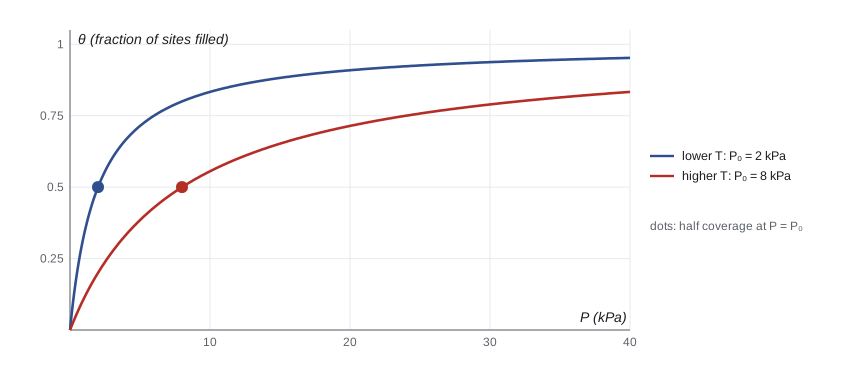
Gas molecules stick to surfaces, an effect central to catalysis, gas storage, gas masks and the sensors in a breathalyzer. Irving Langmuir modelled it in 1918, work that contributed to his 1932 Nobel Prize in Chemistry. Suppose a surface has \(N_s\) independent sites, each of which can hold at most one molecule with binding energy \(-\varepsilon\), in contact with a gas at pressure \(P\) and temperature \(T\). Each site is a grand canonical system exactly like the binding site of lesson 7, so the fraction of occupied sites is

using \(e^{\mu/kT} = n/n_QZ_{\text{int}} = P/(kTn_QZ_{\text{int}})\), with \(Z_{\text{site}}\) the partition function of a molecule's vibrations on its site. At low pressure the coverage is proportional to \(P\); at high pressure it saturates at a full monolayer. The pressure for half coverage, \(P_0\), rises steeply with temperature because of the factor \(e^{-\varepsilon/kT}\): warming a surface releases what it holds, which is how adsorbents are regenerated. Plotting \(1/\theta\) against \(1/P\) gives a straight line, the usual way to test the model against data. Multilayer adsorption, used to measure the surface area of powders, is described by the extension of Brunauer, Emmett and Teller (1938).

Polymers and entropic elasticity

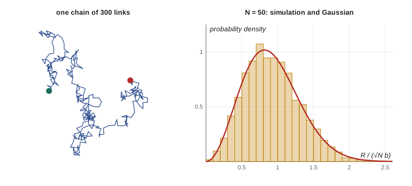
A rubber band is made of long polymer chains, cross-linked into a network. Its elasticity is surprising: it comes almost entirely from entropy, not from stretching chemical bonds. Model one chain as \(N\) links of length \(b\), each pointing in a random direction independently, the freely jointed chain. Its end-to-end vector \(\mathbf R\) is a random walk, so \(\overline{R^2} = Nb^2\), and for large \(N\) the distribution of \(\mathbf R\) is Gaussian with variance \(Nb^2/3\) per component. The number of chain conformations with a given \(\mathbf R\) is therefore proportional to \(e^{-3R^2/2Nb^2}\), and the entropy is

Stretching the chain reduces the number of available conformations and lowers its entropy. At constant temperature the free energy \(F = U - TS\) rises by \(3kTR^2/2Nb^2\) even though \(U\) does not change, so holding the ends apart requires a force

The chain is a Hookean spring with a spring constant proportional to temperature. The fourth part of the program builds 6,000 random chains of 50 links, finds \(\overline{R^2} = 50.3b^2\) against the theoretical 50, and checks the Gaussian shape. For links of 1 nm, the entropic spring constant is about 0.25 pN/nm at 300 K, the scale of forces measured on single DNA and protein molecules with optical tweezers.

Entropic elasticity explains two old observations about rubber, made by John Gough in 1805 and studied by James Joule in the 1850s. A stretched rubber band held at fixed length pulls harder when heated, because its spring constant is proportional to \(T\), the opposite of a metal spring. And a rubber band stretched quickly, without time to exchange heat, warms up, which you can feel by touching it to your lip: the entropy lost by the chains is made up by heating. Thermodynamically, stretching rubber is like compressing a gas, whose pressure is also purely entropic.

Entropy as information

Lesson 4 introduced the Gibbs entropy \(S = -k\sum_ip_i\ln p_i\). In 1948 Claude Shannon, working on communication over noisy channels, defined the information content of a message source in exactly the same form, \(H = -\sum_ip_i\log_2p_i\), measured in bits. The two are the same quantity in different units: \(S = (k\ln 2)H\). The entropy of a macrostate measures how much information would be needed to specify the microstate, given only the macroscopic description.

In 1957 Edwin Jaynes turned this around. He argued that statistical mechanics is a form of inference: given only some average values, such as the mean energy, the least biased probability distribution is the one that maximizes the entropy subject to those constraints. Maximizing \(-\sum p_i\ln p_i\) with a fixed \(\sum p_iE_i\) using a Lagrange multiplier gives \(p_i \propto e^{-\beta E_i}\): the Boltzmann distribution, with \(\beta\) as the multiplier. Jaynes illustrated the idea with a die known only to average 4.5 instead of 3.5. The fifth part of the program finds the maximum-entropy probabilities by bisection on the multiplier: they rise geometrically from 0.054 for a one to 0.348 for a six, carrying 2.33 bits of uncertainty instead of the 2.58 of a fair die. This view explains why the fundamental postulate works so broadly, and it has spread to fields from image reconstruction to ecology.

The link between information and thermodynamics is physical, not just formal. Rolf Landauer argued in 1961 that erasing one bit of information, resetting a memory to a standard state regardless of its previous contents, reduces the entropy of the memory by \(k\ln2\) and must therefore increase the entropy of the surroundings by at least as much. Erasure must dissipate at least \(kT\ln2\) of heat, \(2.87 \times 10^{-21}\) J at 300 K, as the last line of the output shows. This resolved the paradox of Maxwell's demon, which seemed to beat the second law by sorting molecules: the demon must eventually erase its records, and that costs exactly the entropy it saved. In 2012 Antoine Bérut and colleagues measured the heat released when a single colloidal bead in an optical trap was used as a one-bit memory, and found it approaching the Landauer limit for slow erasures. Modern computer chips dissipate far more than this per operation, but the limit sets a floor that future technologies cannot pass.

Looking back

This course began with counting microstates and the observation that relative fluctuations fall as \(1/\sqrt N\). From that start it derived temperature, pressure and chemical potential; the Boltzmann and Gibbs distributions; the equations of state of gases; the heat capacities of magnets, molecules, metals and crystals; the structure of white dwarfs; the blackbody spectrum; Bose–Einstein condensation; phase transitions and universality; and, in this lesson, chemical equilibrium, stellar ionization, adsorption, rubber elasticity and the thermodynamic cost of information. The same few ideas explained all of them. Statistical mechanics continues in courses on condensed matter (PHYS-410), where electrons in periodic potentials and phonons are treated in depth, and in nonequilibrium physics, where fluctuation theorems discovered since the 1990s extend the second law to small systems far from equilibrium.