The canonical ensemble and the partition function

The microcanonical ensemble is conceptually simple but awkward in practice: it requires counting the microstates at exactly one energy, which forces us to handle constraints like the sphere in momentum space of lesson 3. Most real systems are not isolated anyway. A sample in a laboratory sits in contact with its surroundings and exchanges energy with them, so its temperature, not its energy, is what is held fixed. The canonical ensemble describes exactly this situation, and it turns out to be far easier to calculate with. Its central object is the partition function \(Z\), a single sum over states from which every thermodynamic quantity follows. This lesson derives the Boltzmann distribution carefully, builds the machinery of the partition function and the Helmholtz free energy, and shows that energy fluctuations in the canonical ensemble are tied to the heat capacity.

The Boltzmann distribution from a reservoir

Let a small system S be in thermal contact with a large reservoir R, the two together forming an isolated whole of energy \(U_0\). Ask: what is the probability that S is in one particular microstate \(s\) with energy \(E_s\)? The combined system obeys the fundamental postulate, so the probability is proportional to the number of microstates of the whole that have S in state \(s\). That number is simply the multiplicity of the reservoir with energy \(U_0 - E_s\):

Because the reservoir is large, \(E_s\) is a tiny fraction of its energy, and we can expand its entropy to first order:

The second-order term involves \(\partial(1/T)/\partial U\), which is inversely proportional to the reservoir's heat capacity and vanishes for a large enough reservoir. The first term is the same for every state of S and cancels on normalization. Therefore

This is the Boltzmann distribution, and \(Z\) is the partition function. The derivation used nothing about S except that it is small compared with the reservoir, so it applies to a single atom, a molecule, a spin, or a macroscopic sample in a much larger bath. The sum runs over microstates, not energy levels: a level with degeneracy \(g\) contributes \(g\,e^{-E/kT}\). It is common to write \(\beta = 1/kT\).

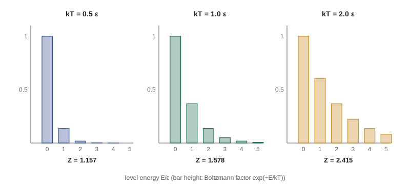
The partition function has a direct meaning: it is approximately the number of states that are thermally accessible. At low temperature only the ground state contributes and \(Z \approx 1\) (if the ground state is not degenerate); at high temperature many states contribute and \(Z\) is large.

Averages from the partition function

The mean energy is \(\bar E = \sum_s E_s P(s)\). Differentiating \(Z\) with respect to \(\beta\) brings down a factor of \(-E_s\) from each term, so

This trick is the main reason the partition function is useful: every average can be written as a derivative of \(\ln Z\). Differentiating again gives the mean square energy, \(\overline{E^2} = Z^{-1}\partial^2 Z/\partial\beta^2\), and therefore the variance:

The last step uses \(\partial/\partial\beta = -kT^2\,\partial/\partial T\) and \(C_V = \partial\bar E/\partial T\). This is a first example of a fluctuation–dissipation relation: the size of spontaneous fluctuations in equilibrium is fixed by a response coefficient, here the heat capacity. Since \(C_V \propto N\) and \(\bar E \propto N\), the relative fluctuation \(\sigma_E/\bar E\) is of order \(1/\sqrt N\), which is why the canonical and microcanonical ensembles agree for macroscopic systems.

The Helmholtz free energy

Thermodynamics introduces the Helmholtz free energy \(F = U - TS\), the potential that is minimized for a system at fixed temperature and volume. The connection to statistical mechanics is the most important formula of the canonical ensemble:

To prove it, compute the entropy from the probabilities. Gibbs's formula for the entropy of any probability distribution over microstates is \(S = -k\sum_s P(s)\ln P(s)\), which reduces to \(k\ln\Omega\) when all \(\Omega\) states are equally likely. With the Boltzmann distribution, \(\ln P(s) = -\beta E_s - \ln Z\), so

and rearranging gives \(\bar E - TS = -kT\ln Z\). Once \(F(T, V, N)\) is known, everything else follows from the thermodynamic identity \(dF = -S\,dT - P\,dV + \mu\,dN\):

The recipe of the canonical ensemble is therefore: list the states, compute \(Z\), take its logarithm, differentiate. No constraint on the total energy has to be imposed, which is what makes the method so much easier than counting at fixed energy.

Checking the formulas numerically

The program below works with a small system of four states with energies 0, \(\varepsilon\), \(\varepsilon\) and \(3\varepsilon\) (a doubly degenerate level appears twice). It computes \(Z\), the mean energy, the variance, the heat capacity by numerical differentiation, the Gibbs entropy and \((U - F)/T\). The columns for \(\sigma_E^2\) and \(kT^2C\) agree, as do the two entropies. At high temperature the entropy approaches \(k\ln 4\), with all four states equally populated.

import math

# A small system: energy levels in units of eps (degenerate levels listed twice)
levels = [0.0, 1.0, 1.0, 3.0]

def stats(kT):
    b = 1 / kT
    w = [math.exp(-b * e) for e in levels]
    Z = sum(w)
    p = [x / Z for x in w]
    U = sum(pi * e for pi, e in zip(p, levels))
    U2 = sum(pi * e * e for pi, e in zip(p, levels))
    F = -kT * math.log(Z)
    S_gibbs = -sum(pi * math.log(pi) for pi in p)          # in units of k
    return Z, U, U2 - U * U, F, S_gibbs

print("Four states with energies 0, 1, 1, 3 (units of eps); k = 1")
print("  kT     Z       <E>     var(E)   kT^2 C   S(Gibbs)  (U-F)/T")
for kT in (0.25, 0.5, 1.0, 2.0, 10.0):
    Z, U, var, F, S = stats(kT)
    h = 1e-5
    C = (stats(kT + h)[1] - stats(kT - h)[1]) / (2 * h)      # dU/dT
    print(f"  {kT:<5}  {Z:6.4f}  {U:6.4f}  {var:7.4f}  {kT * kT * C:7.4f}  {S:7.4f}   {(U - F) / kT:7.4f}")

# <E> = -d ln Z / d beta, checked by finite difference at kT = 1
b, h = 1.0, 1e-6
lnZ = lambda b: math.log(sum(math.exp(-b * e) for e in levels))
print(f"\n  -d ln Z/d beta at kT = 1: {-(lnZ(b + h) - lnZ(b - h)) / (2 * h):.4f}  (matches <E> above)")

# Relative energy fluctuation of a macroscopic Einstein solid at kT = eps
N = 6.022e23
x = 1.0                                   # eps/kT
u = 1 / (math.exp(x) - 1)                 # mean quanta per oscillator
c = x * x * math.exp(x) / (math.exp(x) - 1) ** 2   # C/(Nk)
rel = math.sqrt(N * c) / (N * u)          # sigma_E / U with k = eps = T = 1
print(f"  one mole of oscillators at kT = eps: sigma_E/U = {rel:.2e}")

Four states with energies 0, 1, 1, 3 (units of eps); k = 1
  kT     Z       <E>     var(E)   kT^2 C   S(Gibbs)  (U-F)/T
  0.25   1.0366  0.0354   0.0341   0.0341   0.1774    0.1774
  0.5    1.2731  0.2184   0.1824   0.1824   0.6784    0.6784
  1.0    1.7855  0.4957   0.4173   0.4173   1.0754    1.0754
  2.0    2.4362  0.7727   0.7252   0.7252   1.2768    1.2768
  10.0   3.5505  1.1357   1.0979   1.0979   1.3807    1.3807

  -d ln Z/d beta at kT = 1: 0.4957  (matches <E> above)
  one mole of oscillators at kT = eps: sigma_E/U = 2.12e-12

The last line estimates the energy fluctuation of a mole of oscillators: a relative size of about \(2 \times 10^{-12}\). A macroscopic body in a heat bath has, for all practical purposes, a definite energy.

Independent subsystems and identical particles

If a system consists of two independent parts whose energies add, \(E = E_a + E_b\), each microstate is a pair of states and the Boltzmann factor factorizes. The partition function becomes a product, \(Z = Z_aZ_b\), and the free energies add. This is the second great convenience of the canonical ensemble. For \(N\) distinguishable, independent, identical subsystems, such as the oscillators of an Einstein solid or the spins of a paramagnet, \(Z = Z_1^N\), where \(Z_1\) is the partition function of one subsystem.

For \(N\) indistinguishable particles of a dilute gas, the product \(Z_1^N\) overcounts each microstate \(N!\) times, as in lesson 3, so

This is an approximation valid when there are far more single-particle states thermally available than particles, so that two particles rarely occupy the same state; lesson 8 shows exactly when it fails and what replaces it. For a single atom in a box the sum over states can be replaced by an integral over phase space, \(Z_1 = h^{-3}\int d^3x\,d^3p\,e^{-p^2/2mkT} = V/\lambda^3\). Then \(F = -kT\ln(Z_1^N/N!)\) reproduces the Sackur–Tetrode entropy and the ideal gas law in a few lines, which lesson 6 carries out.

The Einstein solid in the canonical ensemble

The contrast with lessons 2 and 3 is instructive. There, finding the temperature of an Einstein solid required counting the ways to distribute \(q\) quanta, using Stirling's approximation and differentiating. In the canonical ensemble each oscillator is an independent subsystem with levels \(n\varepsilon\), so

Then \(\ln Z = -N\ln(1 - e^{-\beta\varepsilon})\), and one derivative gives \(\bar E = N\varepsilon/(e^{\beta\varepsilon} - 1)\), the same result in two lines. A second derivative gives the heat capacity,

which approaches \(Nk\) at high temperature and vanishes exponentially at low temperature. For a real solid of \(N_a\) atoms, \(N = 3N_a\) and the high-temperature limit is \(3N_ak\), the law of Dulong and Petit (1819). The exponential fall-off was Einstein's explanation of why diamond has a small heat capacity at room temperature; lesson 10 shows why the real fall-off is a gentler \(T^3\).

Equivalence of the ensembles

The canonical ensemble lets the energy fluctuate, while the microcanonical fixes it. For a macroscopic system the canonical energy distribution is \(P(E) \propto \Omega(E)e^{-E/kT}\): a steeply rising multiplicity times a steeply falling exponential, whose product is a spike at the energy where \(\partial\ln\Omega/\partial E = 1/kT\), the microcanonical temperature. The width of the spike is \(\sigma_E = \sqrt{kT^2C}\), which is negligible for large \(N\). Evaluating \(Z = \sum_E\Omega(E)e^{-E/kT}\) by its largest term gives \(\ln Z \approx \ln\Omega - \bar E/kT\), so \(F = \bar E - TS\) with \(S = k\ln\Omega\): the two ensembles give the same thermodynamics. They differ only for small systems, or near phase transitions where the heat capacity becomes enormous.

Where the partition function comes from in practice

Real calculations combine the factorization rules. A molecule's energy is, to a good approximation, a sum of translational, rotational, vibrational, electronic and nuclear-spin parts, so its single-molecule partition function is a product \(Z_1 = Z_{\text{tr}}Z_{\text{rot}}Z_{\text{vib}}Z_{\text{el}}Z_{\text{nuc}}\), and \(\ln Z\) is a sum of separate contributions. Each contribution to the heat capacity can be calculated on its own and added. Lessons 5 and 6 apply this to magnets and molecular gases.