
PHYS-361 · Lesson 11 of 12 · 21 min
Phase transitions and critical phenomena: Ising model, mean-field theory and universality
Everything so far has concerned particles that do not interact, or interact only weakly. That is why the partition functions factorized and the calculations were exact. Phase transitions, such as water freezing, a magnet losing its magnetization at the Curie point, or a fluid reaching its critical point, are collective phenomena that exist only because particles interact. They pose the hardest problems in statistical mechanics, because the partition function no longer factorizes. This lesson studies the simplest model that has a phase transition, the Ising model, using three approaches: exact solutions where they exist, the mean-field approximation, and Landau's general theory. It ends with the remarkable discovery that very different systems behave identically near their critical points, an idea called universality. The capstone of PHYS-234 simulated the Ising model with the Metropolis algorithm; here we focus on the theory that explains those simulations.
The Ising model
Place a spin \(s_i = \pm1\) on each site of a lattice. Neighbouring spins interact with energy \(-J\) if they are parallel and \(+J\) if antiparallel, with \(J > 0\) favouring alignment, and each spin couples to an external field with energy \(-Bs_i\) (absorbing the moment into \(B\)):
where the first sum runs over nearest-neighbour pairs. Wilhelm Lenz proposed the model in 1920 as a picture of a ferromagnet, and his student Ernst Ising solved it in one dimension in 1925. It is a caricature of iron, but the same mathematics describes alloys whose atoms order on a lattice, a lattice gas whose sites are full or empty (and hence the liquid–gas transition), and much else. At low temperature the energy wins and the spins align, giving a spontaneous magnetization even with \(B = 0\). At high temperature the entropy wins and the spins are disordered. A phase transition, if there is one, separates the two at a critical temperature \(T_c\).
One dimension: no transition
In one dimension the model can be solved exactly with the transfer-matrix method. For a ring of \(N\) spins the partition function is the trace of the \(N\)th power of a 2 by 2 matrix, and for large \(N\) it is dominated by the largest eigenvalue, \(\lambda_+ = e^{\beta J}\cosh\beta B + \sqrt{e^{2\beta J}\sinh^2\beta B + e^{-2\beta J}}\). Differentiating \(\ln\lambda_+\) with respect to \(B\) gives the magnetization, which vanishes as \(B \to 0\) at every temperature above zero. Ising concluded, correctly, that his chain has no phase transition, and incorrectly guessed that no dimension would.
The reason is simple. In one dimension a single broken bond, costing energy \(2J\), splits an aligned chain into two oppositely aligned domains, and the broken bond can sit at any of \(N\) places, gaining entropy \(k\ln N\). For large \(N\) the entropy always wins, so long-range order is destroyed at any \(T > 0\). The spins remain correlated over a correlation length \(\xi = -1/\ln\tanh(\beta J)\) lattice sites, which grows very rapidly as \(T\) falls but stays finite. The program computes it: 27 sites at \(kT = J/2\), 3.7 sites at \(kT = J\).
Two dimensions: Onsager's solution
In two dimensions the domain-wall argument fails. A domain of size \(L\) costs an energy proportional to its perimeter, of order \(JL\), while the number of shapes it can take grows only exponentially in \(L\). Rudolf Peierls showed in 1936 that at low enough temperature the energy cost wins and long-range order survives. In 1944 Lars Onsager solved the two-dimensional model on a square lattice exactly in zero field, a mathematical tour de force. The critical temperature satisfies \(\sinh(2J/kT_c) = 1\), giving
and the spontaneous magnetization, announced by Onsager and proved by Chen Ning Yang in 1952, is
The heat capacity diverges logarithmically at \(T_c\), and the magnetization vanishes as \((T_c - T)^{1/8}\). No exact solution is known in three dimensions; there, the critical properties come from numerical simulation and from the renormalization group.
Mean-field theory
Pierre Weiss in 1907 proposed a simple approximation that captures the essence of ordering. Focus on one spin. Its energy is \(-s_i(J\sum_js_j + B)\), where the sum runs over its \(z\) neighbours. Replace each neighbour by its average value \(m\), ignoring fluctuations. The spin then sits in an effective field \(B_{\text{eff}} = zJm + B\), and as an independent spin in a field, lesson 5 gives its average \(m = \tanh(\beta B_{\text{eff}})\). Self-consistency requires
In zero field, \(m = 0\) is always a solution. A nonzero solution exists when the slope of \(\tanh(\beta zJm)\) at the origin exceeds 1, that is when \(\beta zJ > 1\), so the mean-field critical temperature is \(kT_c = zJ\). Near \(T_c\), expanding \(\tanh x \approx x - x^3/3\) gives \(m^2 \approx 3(T_c - T)/T_c\), so
Above \(T_c\), the susceptibility \(\partial m/\partial B\) follows the Curie–Weiss law \(\chi \propto 1/(T - T_c)\), which diverges at the transition. The program solves the self-consistency equation by iteration for a square lattice (\(z = 4\)) and compares with Onsager's exact result. Mean-field theory predicts \(T_c = 4J/k\), far above the true 2.269, because neglecting fluctuations overestimates order; it gets the qualitative picture right but the critical behaviour wrong. The fitted exponents make the point: about 0.5 for mean field, 0.125 for the exact solution.
import math, random
rnd = random.Random(361)

# 1. Mean-field (Weiss) theory: m = tanh(z J m / kT), units J = k = 1
def mf(T, z=4):
    m = 1.0
    for _ in range(20000):
        new = math.tanh(z * m / T)
        if abs(new - m) < 1e-13: break
        m = new
    return m

# 2. Exact spontaneous magnetization of the 2D square-lattice Ising model (Onsager, Yang)
Tc_exact = 2 / math.log(1 + math.sqrt(2))
def exact(T):
    return (1 - math.sinh(2 / T) ** -4) ** 0.125 if T < Tc_exact else 0.0

print(f"square lattice, z = 4: mean-field Tc = 4, exact Tc = 2/ln(1+sqrt 2) = {Tc_exact:.4f}")
print("   T     mean-field m   exact m")
for T in (1.0, 1.5, 2.0, 2.2, 2.26, 2.5, 3.0, 3.5, 3.9):
    print(f"  {T:5}    {mf(T):.4f}        {exact(T):.4f}")

# critical exponent beta from the slope of ln m against ln(Tc - T)
for name, f, tc in (('mean-field', mf, 4.0), ('exact 2D', exact, Tc_exact)):
    t1, t2 = 1e-4, 1e-3
    b = (math.log(f(tc * (1 - t2))) - math.log(f(tc * (1 - t1)))) / math.log(t2 / t1)
    print(f"  {name}: m ~ (Tc - T)^beta with beta = {b:.4f}")

# 3. 1D Ising chain by the transfer matrix: no spontaneous magnetization at any T > 0
def chain_m(T, B):
    b = 1 / T
    return math.exp(b) * math.sinh(b * B) / math.sqrt(math.exp(2 * b) * math.sinh(b * B) ** 2 + math.exp(-2 * b))
print("\n1D chain: magnetization in a tiny field B = 1e-6 (J = 1)")
for T in (0.5, 1.0, 2.0):
    xi = -1 / math.log(math.tanh(1 / T))
    print(f"  T = {T}: m = {chain_m(T, 1e-6):.2e}, correlation length {xi:.1f} sites")

# 4. A quick Metropolis check on a 16 x 16 lattice
L = 16
def run(T, sweeps=1500, burn=500):
    s = [[1] * L for _ in range(L)]
    acc = []
    for sw in range(sweeps):
        for _ in range(L * L):
            i, j = rnd.randrange(L), rnd.randrange(L)
            nb = s[(i + 1) % L][j] + s[i - 1][j] + s[i][(j + 1) % L] + s[i][j - 1]
            dE = 2 * s[i][j] * nb
            if dE <= 0 or rnd.random() < math.exp(-dE / T):
                s[i][j] = -s[i][j]
        if sw >= burn:
            acc.append(abs(sum(map(sum, s))) / (L * L))
    return sum(acc) / len(acc)
print("\nMetropolis, 16 x 16, |m| averaged over 1000 sweeps")
for T in (2.0, 2.27, 2.6):
print(f" T = {T}: simulation {run(T):.3f}, exact infinite lattice {exact(T):.3f}")square lattice, z = 4: mean-field Tc = 4, exact Tc = 2/ln(1+sqrt 2) = 2.2692
T mean-field m exact m
1.0 0.9993 0.9993
1.5 0.9899 0.9865
2.0 0.9575 0.9113
2.2 0.9355 0.7848
2.26 0.9278 0.6134
2.5 0.8906 0.0000
3.0 0.7755 0.0000
3.5 0.5811 0.0000
3.9 0.2711 0.0000
mean-field: m ~ (Tc - T)^beta with beta = 0.4958
exact 2D: m ~ (Tc - T)^beta with beta = 0.1249
1D chain: magnetization in a tiny field B = 1e-6 (J = 1)
T = 0.5: m = 1.09e-04, correlation length 27.3 sites
T = 1.0: m = 7.39e-06, correlation length 3.7 sites
T = 2.0: m = 1.36e-06, correlation length 1.3 sites
Metropolis, 16 x 16, |m| averaged over 1000 sweeps
T = 2.0: simulation 0.910, exact infinite lattice 0.911
T = 2.27: simulation 0.700, exact infinite lattice 0.000
T = 2.6: simulation 0.297, exact infinite lattice 0.000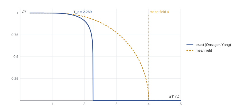
The small Metropolis simulation at the end of the program shows two things. Well below \(T_c\) the 16 by 16 lattice reproduces the exact magnetization. At and above \(T_c\) it shows a nonzero average \(|m|\), because a finite lattice cannot have a sharp transition: fluctuations of order \(1/\sqrt{\text{size}}\) remain. The PHYS-234 capstone studied these finite-size effects and the slowing of the simulation near \(T_c\) in detail.
Landau theory
In 1937 Lev Landau proposed a general framework that does not depend on the details of any model. Near a continuous transition, the order parameter \(m\) is small, so the free energy per unit volume can be expanded in powers of \(m\). If the system has an up–down symmetry, only even powers appear:
Above \(T_c\) the coefficient of \(m^2\) is positive and the minimum is at \(m = 0\). Below \(T_c\) it is negative and the free energy has two minima at \(m = \pm m_0\) with \(m_0^2 = a(T_c - T)/2b\): again \(m \propto (T_c - T)^{1/2}\). The system must choose one of the two minima, breaking the symmetry of its own free energy, an example of spontaneous symmetry breaking, an idea that later proved central to particle physics. Landau theory also predicts \(\chi \propto |T - T_c|^{-1}\), a jump in the heat capacity, and \(m \propto B^{1/3}\) at \(T_c\). These are the mean-field critical exponents, and Landau theory is mean-field theory in general form.
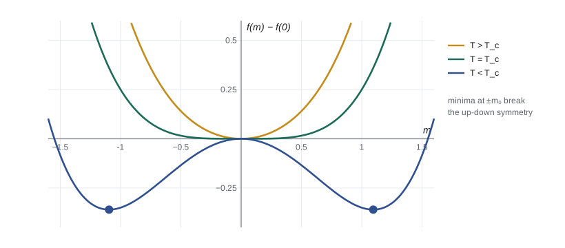
If the expansion contains a cubic term, or if the quartic coefficient is negative (with a positive sixth-order term to keep \(f\) bounded), the order parameter jumps discontinuously and the transition is first order, with latent heat, like melting or boiling. Continuous transitions with a diverging correlation length, like the Curie point, are second order, or critical.
Critical exponents and universality
Near a critical point, measurable quantities follow power laws in \(t = (T - T_c)/T_c\), characterized by critical exponents: \(m \propto |t|^\beta\), \(\chi \propto |t|^{-\gamma}\), \(C \propto |t|^{-\alpha}\), and the correlation length \(\xi \propto |t|^{-\nu}\). Their values reveal something profound:
| Exponent | Mean field | 2D Ising (exact) | 3D Ising (numerical) |
|---|---|---|---|
| \(\beta\) | 1/2 | 1/8 | 0.326 |
| \(\gamma\) | 1 | 7/4 | 1.237 |
| \(\nu\) | 1/2 | 1 | 0.630 |
| \(\alpha\) | 0 (jump) | 0 (logarithm) | 0.110 |
In 1945 Edward Guggenheim plotted the coexisting liquid and vapour densities of eight different substances, from neon to methane, against reduced temperature, and found that they all fell on one curve with the density difference vanishing as \((T_c - T)^{1/3}\), not the mean-field square root. Later measurements on fluids gave \(\beta \approx 0.326\), the same as the three-dimensional Ising magnet. A liquid near its critical point and a uniaxial magnet near its Curie point, utterly different systems, share the same critical exponents. This is universality: critical behaviour depends only on the dimension of space and the symmetry of the order parameter, not on microscopic details. Mean-field theory fails because it ignores fluctuations, which grow without limit near \(T_c\) as the correlation length diverges; mean-field exponents are correct only above four dimensions.
The explanation of universality came from the renormalization group. Leo Kadanoff suggested in 1966 that near \(T_c\) one could group spins into blocks and describe the blocks by an Ising model with new couplings. Kenneth Wilson turned this into a calculational method around 1971: repeatedly coarse-graining the system flows its couplings toward a fixed point that depends only on dimension and symmetry, and the exponents are properties of that fixed point. Wilson received the 1982 Nobel Prize in Physics for this work, which reshaped not only statistical mechanics but particle physics as well.
Worked problem
Mean-field critical temperature
Find the mean-field critical temperature of the Ising model on a simple cubic lattice (\(z = 6\)), and compare with the numerical value \(kT_c = 4.51J\).
Show solution
- Mean field gives \(kT_c = zJ = 6J\).
- The ratio of the exact to the mean-field value is \(4.51/6 = 0.75\).
- In two dimensions the ratio is \(2.269/4 = 0.57\).
Answer: Mean field overestimates \(T_c\) by about a third in three dimensions and by more in two; fluctuations matter less as the number of neighbours grows.
Common mistakes
MistakeExpecting a phase transition in the one-dimensional Ising model.
InsteadDomain walls cost finite energy but gain entropy \(k\ln N\); there is no order at \(T > 0\).
MistakeTrusting mean-field critical exponents in two or three dimensions.
InsteadFluctuations change them: \(\beta = 1/8\) in 2D and about 0.326 in 3D.
MistakeTreating a finite simulation's \(|m|\) above \(T_c\) as genuine order.
InsteadFinite systems have no sharp transition; \(|m|\) falls as \(1/\sqrt{\text{size}}\) above \(T_c\).
MistakeAssuming all transitions are continuous.
InsteadCubic terms or negative quartic terms in the Landau expansion give first-order jumps with latent heat.
Summary and key terms
- The Ising model of interacting spins is the simplest system with a phase transition.
- The 1D chain has no transition; in 2D Onsager found \(kT_c = 2.269J\) and \(m \propto (T_c - T)^{1/8}\).
- Mean-field theory solves \(m = \tanh(\beta(zJm + B))\), giving \(kT_c = zJ\) and \(\beta = 1/2\).
- Landau theory expands the free energy in the order parameter; symmetry and the signs of the coefficients decide the order of the transition.
- Critical exponents are universal, depending only on dimension and symmetry, as the renormalization group explains.
- Ising model
- A lattice of \(\pm1\) spins with nearest-neighbour coupling \(-Js_is_j\).
- Order parameter
- A quantity that is zero in the disordered phase and nonzero in the ordered one, such as \(m\).
- Mean-field theory
- An approximation replacing each neighbour by its average, neglecting fluctuations.
- Critical exponent
- The power in a law such as \(m \propto (T_c - T)^\beta\) near a critical point.
- Universality
- The sharing of critical exponents by systems with the same dimension and order-parameter symmetry.
Practice problems
Work each problem on paper first, then reveal the answer to check.
Solve \(m = \tanh(m\,T_c/T)\) approximately for \(T = 0.9T_c\).
Show answer
\(m^2 \approx 3(1 - 0.9) = 0.3\), so \(m \approx 0.55\) (iteration gives 0.525).
Compute the 1D correlation length at \(kT = 0.25J\).
Show answer
\(\xi = -1/\ln\tanh 4 = 1490\) sites.
Find the location of the minima of \(f = -0.6m^2 + 0.25m^4\).
Show answer
\(m_0^2 = 0.6/(2 \times 0.25) = 1.2\), so \(m_0 = \pm1.10\).
Using \(m \propto (T_c - T)^{1/8}\), by what factor does \(m\) change when \(T_c - T\) is reduced 256-fold?
Show answer
\(256^{-1/8} = 1/2\).
Why does the liquid–gas critical point belong to the Ising universality class?
Show answer
A lattice gas maps onto the Ising model: the density difference is a scalar order parameter with an up–down (particle–hole) symmetry near \(T_c\).
Lesson quiz · 5 questions
Score 60% or more to complete this lesson.
Create a free account to save your progress, take quizzes and earn a certificate.