Lagrangian mechanics: generalized coordinates and constraints

Lesson 1 showed that Hamilton's principle reproduces Newton's law for a single particle in one dimension. This lesson builds the full machinery: Lagrange's equations for any number of generalized coordinates, a derivation from Newton's laws through d'Alembert's principle that shows exactly when they hold, and a recipe for applying them. We then use the recipe on two systems that are awkward with forces, a bead on a spinning hoop and a double pendulum, and check the results numerically.

Constraints and their classification

A constraint restricts the possible configurations or motions of a system. Constraints that can be written as equations among the coordinates and time, \(f(\mathbf r_1, \dots, \mathbf r_N, t) = 0\), are called holonomic. A pendulum rod of fixed length, a bead threaded on a wire, and two particles joined by a rigid bar are holonomic. Each such equation removes one degree of freedom, and with \(k\) of them a system of \(N\) particles has \(n = 3N - k\) generalized coordinates \(q_1, \dots, q_n\), in terms of which every position can be written as \(\mathbf r_i = \mathbf r_i(q_1, \dots, q_n, t)\).

Constraints that depend explicitly on time, such as a bead on a hoop that is being spun, are called rheonomic; those that do not are scleronomic. Constraints that restrict velocities in a way that cannot be integrated to a relation among coordinates, such as rolling without slipping on a plane, are nonholonomic; lesson 5 deals with them. Inequality constraints, such as a particle that must stay outside a sphere, are different again: they hold only while contact lasts, and the bead leaving a hemisphere in lesson 5 is an example.

Virtual displacements and d'Alembert's principle

Constraint forces, such as the tension in a pendulum rod or the normal force from a wire, are generally unknown until the motion is known. The key observation of analytical mechanics is that for ideal constraints these forces do no work in any displacement consistent with the constraints at a fixed instant. Such a displacement is called a virtual displacement \(\delta\mathbf r_i\): an imagined, instantaneous change of configuration that respects the constraints as they are at time \(t\). A frictionless wire pushes perpendicular to itself, and a virtual displacement along the wire is perpendicular to that push, so the work is zero. A rigid rod pulls equally and oppositely on its two ends, and any virtual displacement keeps the rod's length fixed, so the total work is zero.

Write Newton's law for particle \(i\) as \(m_i\ddot{\mathbf r}_i = \mathbf F_i + \mathbf C_i\), separating the applied forces \(\mathbf F_i\) (gravity, springs, electric forces) from the constraint forces \(\mathbf C_i\). Dot with \(\delta\mathbf r_i\) and sum. Since \(\sum_i \mathbf C_i\cdot\delta\mathbf r_i = 0\) for ideal constraints,

This is d'Alembert's principle, published by Jean le Rond d'Alembert in 1743. The constraint forces have vanished. If the \(\delta\mathbf r_i\) were independent we could set each bracket to zero, but they are not, because of the constraints. The cure is to express everything in terms of the independent generalized coordinates.

From d'Alembert to Lagrange

Since \(\mathbf r_i = \mathbf r_i(q, t)\), a virtual displacement (at fixed \(t\)) is \(\delta\mathbf r_i = \sum_j \frac{\partial\mathbf r_i}{\partial q_j}\delta q_j\), where now the \(\delta q_j\) are independent. The applied-force term becomes \(\sum_j Q_j\delta q_j\), with the generalized force

For the inertial term we need two identities. The velocity is \(\dot{\mathbf r}_i = \sum_j \frac{\partial\mathbf r_i}{\partial q_j}\dot q_j + \frac{\partial\mathbf r_i}{\partial t}\), so \(\frac{\partial\dot{\mathbf r}_i}{\partial\dot q_j} = \frac{\partial\mathbf r_i}{\partial q_j}\) (cancellation of dots). And \(\frac{d}{dt}\frac{\partial\mathbf r_i}{\partial q_j} = \frac{\partial\dot{\mathbf r}_i}{\partial q_j}\) (the order of differentiation can be swapped). Using both,

where \(T_i = \tfrac12 m_i\dot{\mathbf r}_i^2\). Summing over particles and using the independence of the \(\delta q_j\) gives one equation for each coordinate:

If the applied forces come from a potential \(V(q, t)\), then \(Q_j = -\partial V/\partial q_j\). Since \(V\) does not depend on the velocities, we can move it inside the first term and write \(L = T - V\):

These are Lagrange's equations, and they are exactly the Euler–Lagrange equations of the action. We have proved Hamilton's principle from Newton's laws for any system with ideal holonomic constraints and potential forces. When some forces are not conservative, such as friction, keep them on the right as \(Q_j\). Magnetic forces, which depend on velocity, can still be included in \(L\) through a velocity-dependent potential, as lesson 9 shows.

The recipe

In practice, solving a problem with Lagrange's equations follows the same steps every time. Choose generalized coordinates that build in the constraints. Write the position of each mass in Cartesian components in terms of those coordinates, differentiate to get the velocities, and assemble \(T = \sum\tfrac12 m_i v_i^2\). Write the potential energy \(V\). Form \(L = T - V\). For each coordinate compute \(\partial L/\partial\dot q_j\), differentiate it with respect to time, compute \(\partial L/\partial q_j\), and set the difference to zero. Finally, look for cyclic coordinates and for time independence, which give conserved quantities without further work.

The quantity \(p_j = \partial L/\partial\dot q_j\) is called the generalized or canonical momentum conjugate to \(q_j\). For a Cartesian coordinate it is the ordinary momentum; for an angle it is an angular momentum; for some other coordinates it has no simple name. Lagrange's equation says \(\dot p_j = \partial L/\partial q_j\), so if \(q_j\) is cyclic, \(p_j\) is conserved.

Example: a bead on a spinning hoop

A bead of mass \(m\) slides without friction on a circular hoop of radius \(R\). The hoop spins at a fixed angular velocity \(\omega\) about its vertical diameter, driven by a motor. Let \(\theta\) be the angle of the bead from the bottom of the hoop. The constraint is rheonomic: the hoop's orientation changes with time, but \(\theta\) alone fixes the bead's position at each instant.

The bead's distance from the axis is \(R\sin\theta\), and it moves with velocity \(R\dot\theta\) along the hoop and \(\omega R\sin\theta\) perpendicular to it. These are at right angles, so \(T = \tfrac12 m(R^2\dot\theta^2 + \omega^2R^2\sin^2\theta)\). The height above the bottom is \(R(1 - \cos\theta)\), so

Then \(\partial L/\partial\dot\theta = mR^2\dot\theta\) and \(\partial L/\partial\theta = mR^2\omega^2\sin\theta\cos\theta - mgR\sin\theta\), giving

Equilibria are where the right side vanishes: \(\theta = 0\) (bottom), \(\theta = \pi\) (top), and, if \(\omega^2 > g/R\), \(\cos\theta_0 = g/(R\omega^2)\). Linearize about each. About \(\theta = 0\), \(\ddot\theta \approx -(g/R - \omega^2)\theta\), stable only if \(\omega < \omega_c = \sqrt{g/R}\), with frequency \(\sqrt{g/R - \omega^2}\). About \(\theta_0\), write \(\theta = \theta_0 + \xi\); differentiating the right side at \(\theta_0\) gives \(\ddot\xi = -\omega^2\sin^2\theta_0\,\xi\), a stable oscillation at frequency \(\Omega = \omega\sin\theta_0\).

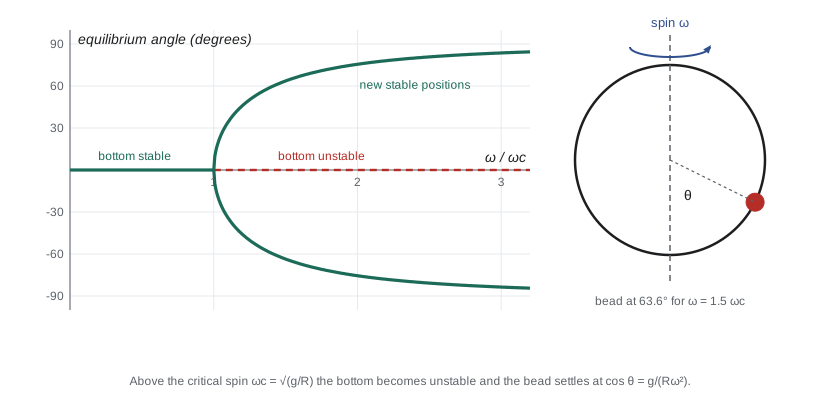
This is a pitchfork bifurcation: as the control parameter \(\omega\) passes \(\omega_c\), one stable equilibrium splits into two stable ones and an unstable one. The bead must choose a side, breaking the left–right symmetry of the hoop. Physically, when the hoop spins fast enough the centrifugal effect, which grows with distance from the axis, beats gravity's pull toward the bottom. The Lagrangian made this easy: we never needed the normal force of the hoop on the bead, which has two components and depends on the motion.

An important subtlety is that the energy \(T + V\) is not conserved here, because the motor does work on the hoop. Yet \(L\) has no explicit \(t\), so the Beltrami quantity \(h = \dot\theta\,\partial L/\partial\dot\theta - L = \tfrac12 mR^2(\dot\theta^2 - \omega^2\sin^2\theta) - mgR\cos\theta\) is conserved. It is not the energy: the term \(\tfrac12 mR^2\omega^2\sin^2\theta\) enters with a minus sign. This conserved quantity, called the energy function or Jacobi integral, equals the energy only when the coordinates are related to Cartesian ones without explicit time dependence.

Example: the double pendulum

Two equal masses \(m\) hang from equal massless rods of length \(\ell\), the second from the first, swinging in a vertical plane. With angles \(\theta_1\), \(\theta_2\) from the vertical, the first mass is at \((\ell\sin\theta_1, -\ell\cos\theta_1)\) and the second at \((\ell\sin\theta_1 + \ell\sin\theta_2, -\ell\cos\theta_1 - \ell\cos\theta_2)\). Squaring the velocities and using \(\cos\theta_1\cos\theta_2 + \sin\theta_1\sin\theta_2 = \cos(\theta_1 - \theta_2)\),

Lagrange's two equations are linear in \(\ddot\theta_1\) and \(\ddot\theta_2\), and solving them gives the expressions used in the program below. With forces this problem requires the tension in both rods and careful bookkeeping of accelerations of a point attached to a moving point; with the Lagrangian it takes half a page. PHYS-244 used the double pendulum as its example of chaos; here we check that our equations are right by testing energy conservation.

import math

def rk4(f, y, dt):
    k1 = f(y); k2 = f([a + dt / 2 * b for a, b in zip(y, k1)])
    k3 = f([a + dt / 2 * b for a, b in zip(y, k2)]); k4 = f([a + dt * b for a, b in zip(y, k3)])
    return [a + dt / 6 * (p + 2 * q + 2 * r + s) for a, p, q, r, s in zip(y, k1, k2, k3, k4)]

# 1. Bead on a hoop of radius R spinning at omega about its vertical diameter.
#    L = (m/2)(R^2 thdot^2 + R^2 omega^2 sin^2 th) + m g R cos th   (th = 0 at the bottom)
#    Lagrange: thddot = sin th (omega^2 cos th - g/R)
g, R = 9.81, 0.20
wc = math.sqrt(g / R)
print(f"critical spin rate sqrt(g/R) = {wc:.3f} rad/s")
for w in (0.8 * wc, 1.5 * wc, 2.5 * wc):
    if w > wc:
        th_eq = math.acos(g / (R * w * w)); Om = w * math.sin(th_eq)          # small-oscillation frequency
    else:
        th_eq = 0.0; Om = math.sqrt(g / R - w * w)
    f = lambda y: [y[1], math.sin(y[0]) * (w * w * math.cos(y[0]) - g / R)]
    y = [th_eq + 0.01, 0.0]; t = 0.0; dt = 1e-4; crossings = []; prev = y[0] - th_eq
    while len(crossings) < 3:
        y = rk4(f, y, dt); t += dt
        cur = y[0] - th_eq
        if prev < 0 <= cur: crossings.append(t)
        prev = cur
    T_num = crossings[2] - crossings[1]
    print(f"omega = {w / wc:.1f} x critical: equilibrium at {math.degrees(th_eq):5.1f} deg, "
          f"period {T_num:.4f} s (formula {2 * math.pi / Om:.4f} s)")

# 2. Double pendulum (equal masses m, equal lengths l) from its Lagrangian; energy must stay constant.
l = 1.0
def dp(y):
    t1, t2, w1, w2 = y; d = t1 - t2
    den = 3 - math.cos(2 * d)
    a1 = (-3 * g * math.sin(t1) - g * math.sin(t1 - 2 * t2) - 2 * math.sin(d) * (w2 * w2 * l + w1 * w1 * l * math.cos(d))) / (l * den)
    a2 = (2 * math.sin(d) * (2 * w1 * w1 * l + 2 * g * math.cos(t1) + w2 * w2 * l * math.cos(d))) / (l * den)
    return [w1, w2, a1, a2]
def energy(y):   # per unit mass
    t1, t2, w1, w2 = y
    T = 0.5 * l * l * (2 * w1 * w1 + w2 * w2 + 2 * w1 * w2 * math.cos(t1 - t2))
    V = -g * l * (2 * math.cos(t1) + math.cos(t2))
    return T + V
y = [math.radians(120), math.radians(-20), 0.0, 0.0]; E0 = energy(y)
dt = 1e-3
for step in range(1, 20001):
    y = rk4(dp, y, dt)
    if step % 5000 == 0:
        print(f"t = {step * dt:4.1f} s: theta1 = {math.degrees(y[0]):8.2f} deg, relative energy error {abs(energy(y) - E0) / abs(E0):.1e}")

critical spin rate sqrt(g/R) = 7.004 rad/s
omega = 0.8 x critical: equilibrium at   0.0 deg, period 1.4952 s (formula 1.4952 s)
omega = 1.5 x critical: equilibrium at  63.6 deg, period 0.6677 s (formula 0.6677 s)
omega = 2.5 x critical: equilibrium at  80.8 deg, period 0.3635 s (formula 0.3635 s)
t =  5.0 s: theta1 =    96.33 deg, relative energy error 1.0e-08
t = 10.0 s: theta1 =   -85.93 deg, relative energy error 1.4e-08
t = 15.0 s: theta1 =   -23.97 deg, relative energy error 1.6e-08
t = 20.0 s: theta1 =    32.57 deg, relative energy error 3.4e-08

For a hoop of radius 0.20 m the critical rate is \(\omega_c = 7.004\ \mathrm{rad/s}\), about 67 revolutions per minute. Below it, the bead oscillates about the bottom with period \(2\pi/\sqrt{g/R - \omega^2}\); above it, about \(\theta_0 = \arccos(g/R\omega^2)\), which is 63.6 degrees at \(1.5\omega_c\) and 80.8 degrees at \(2.5\omega_c\), with period \(2\pi/(\omega\sin\theta_0)\). The periods measured by integrating the full nonlinear equation agree with the linearized formulas to four figures. For the double pendulum released from 120 and \(-20\) degrees, the motion is wild, but the energy stays constant to a few parts in \(10^8\) over 20 s. An error in the equations of motion would show up immediately as energy drift, which makes energy a useful check on any derivation.