Canonical transformations and Hamilton–Jacobi theory

In Lagrangian mechanics we can change coordinates freely and the equations keep their form. Hamiltonian mechanics allows much more: we can mix coordinates and momenta, as long as the new variables still satisfy Hamilton's equations. Such changes of variable are called canonical transformations. Their purpose is to make a problem simple. The ultimate simplification is a set of variables in which the Hamiltonian depends only on momenta, so all momenta are constant and all coordinates advance at constant rates. Finding those variables is the goal of Hamilton–Jacobi theory, and for bounded motion the result is the action-angle variables, which carried classical mechanics into the old quantum theory of Bohr and Sommerfeld and remain the language of perturbation theory for orbits and accelerators.

Canonical transformations

A transformation \((q, p) \to (Q, P)\) is canonical if, for any Hamiltonian \(H(q, p, t)\), there is a function \(K(Q, P, t)\) such that the new variables obey \(\dot Q = \partial K/\partial P\) and \(\dot P = -\partial K/\partial Q\). For transformations that do not depend on time, \(K\) is simply \(H\) rewritten in the new variables. The test is that the transformation preserves the fundamental Poisson brackets:

with the brackets computed in the old variables. For one degree of freedom this reduces to a single condition, that the Jacobian determinant \(\partial(Q, P)/\partial(q, p)\) equals 1: the transformation preserves area in the phase plane, consistent with Liouville's theorem. In more dimensions the condition is stronger than preserving volume; it requires preserving a quantity called the symplectic form, which measures oriented areas projected onto each \((q_j, p_j)\) plane.

Some canonical transformations look surprising. Swapping \(Q = p\), \(P = -q\) is canonical, which shows that in Hamiltonian mechanics there is no deep distinction between coordinates and momenta. A rotation in the phase plane, \(Q = q\cos\alpha + p\sin\alpha\), \(P = -q\sin\alpha + p\cos\alpha\), is canonical. And the time evolution itself, the map taking the state at time 0 to the state at time \(t\), is a canonical transformation, which is another way of stating Liouville's theorem and the reason symplectic integrators work.

Generating functions

Canonical transformations are conveniently produced from a single function. Since both sets of variables must make their phase-space actions stationary, \(\sum p\dot q - H\) and \(\sum P\dot Q - K\) can differ only by a total time derivative \(dF/dt\). Taking \(F\) to depend on the old coordinates and the new momenta, as \(F_2(q, P, t) - \sum QP\), gives the most useful type:

For example, \(F_2 = \sum_j q_jP_j\) gives \(p = P\) and \(Q = q\), the identity. \(F_2 = \sum_j f_j(q)P_j\) gives \(Q_j = f_j(q)\), an arbitrary change of coordinates, with the momenta transforming in the way that keeps the bracket structure. There are three other types, depending on which old and new variables the generating function uses, all related by Legendre transforms.

The Hamilton–Jacobi equation

Now aim for the simplest possible new Hamiltonian, \(K = 0\). Then all new coordinates and momenta are constants, \(Q_j = \beta_j\) and \(P_j = \alpha_j\), and the problem is solved: inverting the transformation gives \(q(t)\) in terms of \(2n\) constants. The condition \(K = 0\) with \(p_j = \partial S/\partial q_j\) is a partial differential equation for the generating function, which is usually called \(S\):

This is the Hamilton–Jacobi equation, set out by Hamilton in 1834 and developed by Carl Jacobi in his lectures of 1842 and 1843. Its solution \(S(q, \alpha, t)\), depending on \(n\) constants \(\alpha\), is called Hamilton's principal function, and it turns out to be the action of lesson 1 evaluated along the true path, as a function of its end point. The motion follows from the equations \(\partial S/\partial\alpha_j = \beta_j\).

When \(H\) does not depend on time, write \(S = W(q, \alpha) - Et\), where \(W\) is Hamilton's characteristic function and \(E\) the energy. Then \(H(q, \partial W/\partial q) = E\). For one degree of freedom with \(H = p^2/2m + V(q)\), this is an ordinary differential equation, \(\frac{1}{2m}(dW/dq)^2 + V = E\), solved by

and the equation \(\partial S/\partial E = \beta\) gives \(\partial W/\partial E = t + \beta\), which is the familiar time integral \(t = \int dq/v\). For the harmonic oscillator the program checks this: \(\partial W/\partial E\) computed numerically at \(q\) equals \(\arcsin(q)\), the time taken on the true motion \(q = \sin t\).

Separation of variables

The Hamilton–Jacobi equation is a single partial differential equation, which sounds harder than Hamilton's \(2n\) ordinary ones. Its power comes from separation of variables. If the Hamiltonian has the right structure, \(W\) can be written as a sum \(W_1(q_1) + W_2(q_2) + \cdots\), and the equation splits into ordinary equations, each introducing a separation constant. Each constant is a conserved quantity. For a central force in spherical coordinates, \(H = \frac{1}{2m}\big(p_r^2 + p_\theta^2/r^2 + p_\phi^2/r^2\sin^2\theta\big) + V(r)\) separates into equations for \(\phi\) (constant \(p_\phi\)), \(\theta\) (constant \(L^2\)) and \(r\) (constant \(E\)). Jacobi used separation in elliptic coordinates to solve the problem of a particle attracted by two fixed centres, which has a conserved quantity with no obvious symmetry behind it. Systems that separate completely are integrable: they have as many independent conserved quantities as degrees of freedom.

Waves and rays

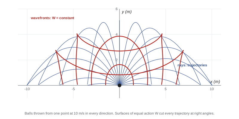
For a fixed energy, the surfaces of constant \(W\) in configuration space behave like wavefronts, and the trajectories, which move along \(\mathbf p = \nabla W\), are perpendicular to them, like light rays crossing the wavefronts of a light wave. Hamilton was led to his mechanics by exactly this analogy with geometrical optics, where the eikonal equation \(|\nabla S|^2 = n^2\) plays the role of the Hamilton–Jacobi equation and the rays are the paths of least time. The analogy was so close that Erwin Schrödinger, in 1926, asked what wave equation would have the Hamilton–Jacobi equation as its short-wavelength limit, in the way that wave optics has geometrical optics as its limit. The answer was his equation. Writing the wavefunction as \(\psi = A\,e^{iS/\hbar}\) and letting \(\hbar \to 0\) turns the Schrödinger equation back into the Hamilton–Jacobi equation.

Action-angle variables

For periodic motion in one degree of freedom there is a particularly useful choice of new momentum, the action variable

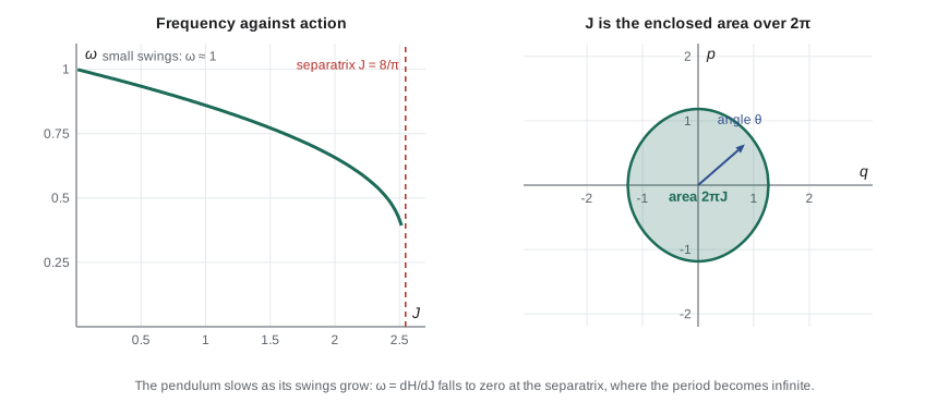
the area enclosed by the orbit in the phase plane, divided by \(2\pi\). Since the orbit is the level curve \(H = E\), \(J\) is a function of \(E\) alone, and conversely \(H = H(J)\). The conjugate coordinate \(\theta\), the angle variable, then obeys \(\dot\theta = \partial H/\partial J = \omega(J)\), a constant, and advances by \(2\pi\) per cycle. So

The frequency of any periodic motion can be found without solving the equations of motion, simply by computing the area of the orbit as a function of energy and differentiating. For the harmonic oscillator, the orbit is an ellipse with semi-axes \(\sqrt{2E/k}\) and \(\sqrt{2mE}\), so \(J = E/\omega_0\) and \(dH/dJ = \omega_0\), independent of amplitude. For the pendulum the frequency falls as the amplitude grows, reaching zero on the separatrix, where \(J = 8/\pi\) in units with \(m = \ell = g = 1\).

In \(n\) dimensions, an integrable system has \(n\) actions \(J_1, \dots, J_n\) and \(n\) angles, and each bounded trajectory winds around an \(n\)-dimensional torus in phase space, with the angles advancing at the frequencies \(\omega_j = \partial H/\partial J_j\). This geometric picture, made rigorous by Joseph Liouville and later by Vladimir Arnold, is the starting point for the theory of chaos in lesson 12.

Adiabatic invariants

Action variables have one more remarkable property. If a parameter of the system, such as the length of a pendulum or the strength of a magnetic field, changes slowly compared with the period, the energy changes but the action stays very nearly constant. A pendulum whose string is slowly shortened speeds up and gains energy, with \(E/\omega\) staying fixed. A charged particle spiralling in a slowly strengthening magnetic field keeps the magnetic flux through its orbit constant, which is why particles are reflected by the strong fields near the Earth's poles and trapped in the Van Allen belts. In the old quantum theory, Paul Ehrenfest used adiabatic invariance in 1916 to explain why quantization should apply to the action: only a quantity that does not change under slow changes could sensibly be restricted to discrete values.

import math

def simpson(f, a, b, n=2000):
    h = (b - a) / n
    return h / 3 * (f(a) + f(b) + sum((4 if k % 2 else 2) * f(a + k * h) for k in range(1, n)))

# 1. Action variable of the pendulum H = p^2/2 - cos q (m = l = g = 1):
#    J(E) = (1/2pi) loop integral of p dq = (2/pi) integral_0^qmax sqrt(2(E + cos q)) dq
def J(E):
    qmax = math.acos(-E)
    # substitute sin(q/2) = k sin(u): then p = 2k cos u and p dq = 4k^2 cos^2 u du / sqrt(1 - k^2 sin^2 u)
    k = math.sin(qmax / 2)
    f = lambda u: 4 * k * k * math.cos(u) ** 2 / math.sqrt(1 - (k * math.sin(u)) ** 2)
    return 2 / math.pi * simpson(f, 0.0, math.pi / 2)
def period_agm(qmax):                      # exact period from the arithmetic-geometric mean
    a, b = 1.0, math.cos(qmax / 2)
    for _ in range(30): a, b = 0.5 * (a + b), math.sqrt(a * b)
    return 2 * math.pi / a
print(" amplitude   J        omega = dE/dJ   2 pi / T(exact)")
for amp_deg in (10, 60, 120, 170):
    qm = math.radians(amp_deg); E = -math.cos(qm); dE = 1e-6
    w = 2 * dE / (J(E + dE) - J(E - dE))
    print(f"  {amp_deg:4d} deg  {J(E):.5f}     {w:.5f}         {2 * math.pi / period_agm(qm):.5f}")

# 2. The harmonic oscillator by Hamilton-Jacobi: W(q, E) = integral sqrt(2(E - q^2/2)) dq and
#    dW/dE = t - t0. Compare with direct integration of the motion.
E = 0.5   # amplitude 1, omega = 1
W = lambda q, E: simpson(lambda s: math.sqrt(max(2 * (E - 0.5 * s * s), 0.0)), 0.0, q)
for q in (0.2, 0.5, 0.8):
    dE = 1e-6; t_hj = (W(q, E + dE) - W(q, E - dE)) / (2 * dE)
    print(f"q = {q}: dW/dE = {t_hj:.6f}; time from q = 0 on the true motion q = sin t is asin(q) = {math.asin(q):.6f}")

# 3. A canonical transformation must preserve Poisson brackets. Test the action-angle map of the
#    oscillator, Q = atan2(q, p) (angle), P = (p^2 + q^2)/2 (action), and a non-canonical map.
def bracket(Qf, Pf, q, p, h=1e-6):
    dQq = (Qf(q + h, p) - Qf(q - h, p)) / (2 * h); dQp = (Qf(q, p + h) - Qf(q, p - h)) / (2 * h)
    dPq = (Pf(q + h, p) - Pf(q - h, p)) / (2 * h); dPp = (Pf(q, p + h) - Pf(q, p - h)) / (2 * h)
    return dQq * dPp - dQp * dPq
for q, p in ((0.3, 0.8), (-1.2, 0.4)):
    good = bracket(lambda q, p: math.atan2(q, p), lambda q, p: 0.5 * (q * q + p * p), q, p)
    bad = bracket(lambda q, p: math.atan2(q, p), lambda q, p: math.sqrt(q * q + p * p), q, p)
    print(f"at (q, p) = ({q}, {p}): {{Q, P}} = {good:.6f} for P = (q^2+p^2)/2, but {bad:.6f} for P = sqrt(q^2+p^2)")

 amplitude   J        omega = dE/dJ   2 pi / T(exact)
    10 deg  0.01521     0.99810         0.99810
    60 deg  0.51732     0.93181         0.93181
   120 deg  1.71105     0.72840         0.72840
   170 deg  2.50461     0.40994         0.40994
q = 0.2: dW/dE = 0.201358; time from q = 0 on the true motion q = sin t is asin(q) = 0.201358
q = 0.5: dW/dE = 0.523599; time from q = 0 on the true motion q = sin t is asin(q) = 0.523599
q = 0.8: dW/dE = 0.927295; time from q = 0 on the true motion q = sin t is asin(q) = 0.927295
at (q, p) = (0.3, 0.8): {Q, P} = 1.000000 for P = (q^2+p^2)/2, but 1.170411 for P = sqrt(q^2+p^2)
at (q, p) = (-1.2, 0.4): {Q, P} = 1.000000 for P = (q^2+p^2)/2, but 0.790569 for P = sqrt(q^2+p^2)

For the pendulum, the program computes \(J(E)\) by quadrature and \(\omega = dE/dJ\) by a numerical derivative, and compares it with \(2\pi/T\), where the exact period comes from the arithmetic-geometric mean as in PHYS-244. They agree to five figures at amplitudes of 10, 60, 120 and 170 degrees, with frequencies of 0.998, 0.932, 0.728 and 0.410. At 170 degrees the action is 2.505, close to the separatrix value \(8/\pi = 2.546\). The Hamilton–Jacobi derivative \(\partial W/\partial E\) reproduces the oscillator's travel times to six figures. Finally, the map \(Q = \operatorname{atan2}(q, p)\), \(P = \tfrac12(q^2 + p^2)\), which takes the unit oscillator to action-angle form, has \(\{Q, P\} = 1\) at every test point, while replacing \(P\) by \(\sqrt{q^2 + p^2}\) gives brackets of 1.17 and 0.79: that map does not preserve area and is not canonical.