Why analytical mechanics: from forces to principles

In PHYS-244 you solved mechanics problems the way Newton did: draw every force, add the vectors, and integrate \(m\ddot{\mathbf r} = \mathbf F\). That approach is direct and always correct, but it becomes clumsy quickly. A bead sliding on a spinning hoop, a double pendulum, a top precessing on a table or a molecule with three vibrating atoms all involve forces you do not know in advance, such as the push of the hoop on the bead or the tension in each rod. Those constraint forces have to be found along with the motion. Coordinates that suit the problem, such as angles, fit awkwardly into a vector equation written in Cartesian components.

This course develops a different way of doing mechanics, built on two ideas. The first is that a mechanical system can be described by any set of numbers that pins down its configuration, called generalized coordinates, and that the equations of motion can be written directly in those coordinates. The second is that the actual motion is singled out by a principle: among all the ways the system could get from one configuration to another in a given time, it takes the one for which a single number, the action, is stationary. From that principle, worked out by Euler, Lagrange and Hamilton between 1744 and 1835, come the Lagrangian and Hamiltonian forms of mechanics, a direct link between symmetries and conservation laws, and the language in which quantum mechanics, statistical mechanics and field theory are written.

What PHYS-244 gave us, and what is missing

PHYS-244 covered drag, rockets, potential energy curves, nonlinear oscillators, central forces and Kepler orbits, rotating frames and rigid bodies, ending with chaos. Several of those topics required effort that the methods of this course remove. The Foucault pendulum needed the Coriolis force worked out in a rotating frame; here it comes out of a short calculation with angles. Euler's equations for a rigid body were derived from the vector form of angular momentum; here we will derive the motion of a heavy symmetric top from a single scalar function. The effective potential for orbits was introduced by hand; in lesson 7 it falls out of the Lagrangian once we notice that one coordinate does not appear in it.

The new methods do not contain new physics. For the systems we study, Lagrange's equations are Newton's second law, rearranged. Their value is practical and conceptual. Practically, they let you write down equations of motion for complicated systems almost mechanically, without ever finding the constraint forces. Conceptually, they show why the laws of mechanics have the form they do, and they reveal structure, such as conserved quantities and the geometry of motion in phase space, that the force picture hides.

Generalized coordinates

The configuration of a system is the set of positions of all its parts. A particle moving freely in space needs three numbers, a pendulum swinging in a plane needs one (the angle), and a double pendulum needs two. The number of independent quantities needed is the number of degrees of freedom. For \(N\) particles subject to \(k\) independent constraint equations there are \(n = 3N - k\) degrees of freedom. Any set of \(n\) numbers \(q_1, \dots, q_n\) that fixes the configuration uniquely is a set of generalized coordinates. They need not be lengths: angles, arc lengths, or the amplitudes of vibration modes all qualify.

For a plane pendulum of length \(\ell\), the bob's Cartesian position \((x, y)\) obeys the constraint \(x^2 + y^2 = \ell^2\). Instead of carrying two coordinates and a constraint, we use one angle \(\theta\) with \(x = \ell\sin\theta\), \(y = -\ell\cos\theta\). The constraint is now built in: every value of \(\theta\) gives a permitted position. This is the essential trick of analytical mechanics, and lessons 4 and 5 treat it in detail.

The action

Consider a single particle of mass \(m\) moving along a line in a potential \(V(x)\). Define the Lagrangian as kinetic minus potential energy,

and the action of a path \(x(t)\) that starts at \(x_1\) at time \(t_1\) and ends at \(x_2\) at time \(t_2\) as

The square brackets are a reminder that \(S\) is not a function of a number but of a whole path; it assigns a number to each possible way of getting from the start to the finish. Such an object is called a functional. The action has the units of energy times time, joule seconds, the same units as Planck's constant.

Hamilton's principle states that the path the particle actually follows is the one for which \(S\) is stationary: if the path is changed by a small amount \(\delta x(t)\) that vanishes at both ends, the change in \(S\) is zero to first order. In lesson 2 we show that this condition is equivalent to the Euler–Lagrange equation

For \(L = \tfrac12 m\dot x^2 - V(x)\), the first term is \(\frac{d}{dt}(m\dot x) = m\ddot x\) and the second is \(-V'(x)\), so the equation reads \(m\ddot x = -V'(x)\): Newton's second law for a conservative force. The principle of stationary action contains Newtonian mechanics.

A numerical experiment

Before proving anything, it is worth seeing the principle work. Divide the time interval into small steps, represent a path by its positions at those times, and approximate the action by a sum. Then start from a wrong guess and move the intermediate points downhill in \(S\) until it stops changing. If the principle is right, the path we arrive at is the one Newton's law predicts.

import math

# Discretized action S = sum over steps of (m/2) v^2 dt - V dt, with both ends fixed.
def action(x, dt, m, V):
    S = 0.0
    for i in range(len(x) - 1):
        v = (x[i + 1] - x[i]) / dt
        xm = 0.5 * (x[i] + x[i + 1])
        S += (0.5 * m * v * v - V(xm)) * dt
    return S

def relax(x, dt, m, dV, sweeps=20000, rate=0.45):
    # gradient descent on the interior points; dS/dx_i = -m(x_{i+1} - 2x_i + x_{i-1})/dt - V'(x_i) dt
    x = list(x)
    for _ in range(sweeps):
        for i in range(1, len(x) - 1):
            grad = -m * (x[i + 1] - 2 * x[i] + x[i - 1]) / dt - dV(x[i]) * dt
            x[i] -= rate * grad * dt / m
    return x

# 1. Free fall: a ball thrown up and caught 2 s later at the same height
m, g, T, N = 1.0, 9.81, 2.0, 40
dt = T / N
V = lambda y: m * g * y; dV = lambda y: m * g
guess = [0.0] * (N + 1)                      # start from "the ball just sits there"
best = relax(guess, dt, m, dV)
exact = [0.5 * g * (i * dt) * (T - i * dt) for i in range(N + 1)]
print("free fall, top of path from minimizing S:", round(max(best), 4), "m; exact", round(max(exact), 4), "m")
print("largest deviation from the exact parabola:", f"{max(abs(a - b) for a, b in zip(best, exact)):.2e} m")

# 2. Varying the true path by eps*sin(pi t/T): S changes only at second order in eps
for eps in (0.0, 0.1, 0.2, 0.4):
    path = [y + eps * math.sin(math.pi * i / N) for i, y in enumerate(exact)]
    print(f"eps = {eps:.1f}: S = {action(path, dt, m, V):.5f} J s")

# 3. Harmonic oscillator: the true path minimizes S only if T < pi/omega
k = 1.0; omega = 1.0
Vh = lambda x: 0.5 * k * x * x
for T in (0.8 * math.pi, 1.2 * math.pi):
    dt = T / N
    true = [math.sin(omega * i * dt) / math.sin(omega * T) * 0.5 for i in range(N + 1)]  # x(0)=0, x(T)=0.5
    S0 = action(true, dt, m, Vh)
    bump = [x + 0.05 * math.sin(math.pi * i / N) for i, x in enumerate(true)]
    print(f"T = {T / math.pi:.1f} pi: S(true) = {S0:.5f}, S(true + bump) = {action(bump, dt, m, Vh):.5f}",
          "-> minimum" if action(bump, dt, m, Vh) > S0 else "-> saddle, not a minimum")

free fall, top of path from minimizing S: 4.905 m; exact 4.905 m
largest deviation from the exact parabola: 5.86e-14 m
eps = 0.0: S = -32.05865 J s
eps = 0.1: S = -32.04632 J s
eps = 0.2: S = -32.00933 J s
eps = 0.4: S = -31.86136 J s
T = 0.8 pi: S(true) = -0.17175, S(true + bump) = -0.17083 -> minimum
T = 1.2 pi: S(true) = 0.17306, S(true + bump) = 0.17224 -> saddle, not a minimum

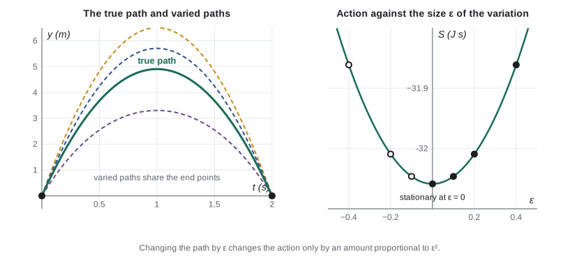
Three things come out of this program. First, starting from a ball that just sits on the ground, gradient descent on the action finds the parabola of a ball thrown up and caught 2 s later, peaking at \(gT^2/8 = 4.905\ \mathrm m\), and agrees with it to rounding error. No force was ever computed: the program only knew the kinetic and potential energy. Second, when the true path is changed by \(\varepsilon\sin(\pi t/T)\), the action rises by an amount proportional to \(\varepsilon^2\): 0.012 for \(\varepsilon = 0.1\), 0.049 for 0.2 and 0.197 for 0.4, a ratio of very nearly four each time \(\varepsilon\) doubles. A first-order change in the path produces only a second-order change in \(S\). That is what stationary means.

Third, stationary does not always mean minimum. For the harmonic oscillator the true path is a minimum of the action only if the time interval is shorter than half a period, \(T < \pi/\omega\). For a longer interval the program finds a variation that lowers the action, so the true path is a saddle point: a minimum along some directions in the space of paths and a maximum along others. That is why the precise statement is the principle of stationary action, not least action. The name least action survives from history, and for short enough time intervals it is accurate.

Why a principle?

It can seem strange that a particle should know about a whole path, including its end point, before it gets there. It does not. The Euler–Lagrange equation is a local differential equation: the acceleration at each instant depends only on the position and velocity at that instant. The variational principle is an equivalent global way of stating the same law, just as the statement that light takes the quickest route between two points (Fermat's principle, which we meet in lesson 2) is equivalent to the local law of refraction at each surface.

The deeper reason the action matters came in 1948, when Richard Feynman showed that quantum mechanics can be built from it. In Feynman's path integral a quantum particle explores every path, each contributing a complex number of size one and phase \(S/\hbar\). For everyday objects the action of a typical path is around \(10^{30}\) or more times \(\hbar\), so the phases of neighbouring paths swing wildly and cancel, except near a path where \(S\) is stationary: there neighbouring paths have nearly the same phase and add up. Classical mechanics is the stationary-phase limit of quantum mechanics. We return to this in lesson 12.

A short history

Pierre de Fermat proposed in 1662 that light travels between two points along the path of least time. Johann Bernoulli posed the brachistochrone problem in 1696, asking for the curve of quickest descent; its solution by several mathematicians, including Newton, launched the calculus of variations. Pierre-Louis Moreau de Maupertuis proposed a principle of least action for mechanics in 1744, and in the same year Leonhard Euler gave it a correct mathematical form for a particle moving in a plane. Joseph-Louis Lagrange developed Euler's methods into the general calculus of variations in a letter to Euler in 1755 and then rewrote all of mechanics in his Mécanique analytique of 1788, a book that famously contained no diagrams.

William Rowan Hamilton, working in Dublin, stated the principle in its modern form in 1834 and 1835 and introduced the equations that bear his name, which treat position and momentum on an equal footing. Carl Jacobi refined Hamilton's work in the 1830s and 1840s, producing the Hamilton–Jacobi equation. Siméon Denis Poisson introduced the bracket that now carries his name in 1809, and Joseph Liouville proved his theorem on phase-space volume in 1838. In 1918 Emmy Noether proved that every continuous symmetry of the action gives a conserved quantity, and at the end of the nineteenth century Henri Poincaré, followed in the twentieth by Kolmogorov, Arnold and Moser, used the Hamiltonian framework to understand when orbits are regular and when they are chaotic.

The plan of the course

Lessons 2 and 3 develop the calculus of variations, the mathematics of finding a function that makes an integral stationary, and apply it to classic problems: the brachistochrone, the hanging chain and the shortest path on a surface. Lessons 4 to 8 build Lagrangian mechanics: generalized coordinates, constraints and the forces that enforce them, Noether's theorem, central forces and the symmetric top, and small oscillations about equilibrium solved as an eigenvalue problem. Lessons 9 to 11 develop Hamiltonian mechanics: Hamilton's equations, phase space and Liouville's theorem, Poisson brackets, canonical transformations, action-angle variables and the Hamilton–Jacobi equation. Lesson 12 draws the threads together and shows how they lead into chaos, quantum mechanics and field theory.

Every lesson has a short program, written with only the Python standard library, that checks the mathematics numerically. Several of them integrate equations of motion with the fourth-order Runge–Kutta method from PHYS-244; from lesson 9 on we will also use the leapfrog method, which respects the geometric structure of Hamiltonian mechanics and so keeps energy errors bounded over very long runs.

Using the methods well

Lagrangian mechanics is most useful when constraints are present and when natural coordinates are not Cartesian. For a single particle in a simple force field, Newton's law is just as quick. Its power appears in problems such as a pendulum hanging from a moving support, a bead on a rotating wire, coupled oscillators, or a top. In each case you write down the kinetic and potential energies in whatever coordinates are convenient, form \(L = T - V\), and the equations of motion follow by differentiation. Because \(T\) and \(V\) are scalars, there is no need to resolve vectors or to keep track of the direction of every force.

A second strength is that energies are often easy to write even when forces are not. The kinetic energy of a rigid body, of a fluid element, or of an electromagnetic field has a compact expression. The Lagrangian approach carries over unchanged to these systems, which is one reason it became the standard language of theoretical physics.