Photon interactions

Back at the Darlington project office, Lina hands Hana a real problem for the tenth session. A caesium-137 calibration source used by the plant's radiation protection technicians gives a dose rate of about 400 µSv/h at 1 m, and the storage cabinet must reduce it to 2.5 µSv/h at its surface position. How much lead does the cabinet need? Answering properly requires the three ways photons interact with matter, the exponential attenuation law and the correction for scattered photons that a narrow-beam calculation misses.

Photons are different again

Gamma rays and X-rays are photons: uncharged packets of electromagnetic energy. Like neutrons, they travel some distance without losing energy and then interact in a single event in which they are absorbed or scattered. Unlike neutrons, they interact mainly with atomic electrons, so their interactions depend strongly on the atomic number and density of the material. Gamma rays from nuclear decay range from tens of keV to about 3 MeV; capture gamma rays from neutron absorption reach about 10 MeV; and the 6.1 and 7.1 MeV gammas of nitrogen-16 (Lesson 4) are among the most penetrating in a reactor.

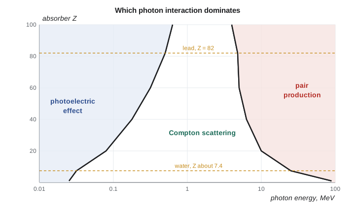
Three interactions dominate between about 10 keV and 10 MeV: the photoelectric effect, Compton scattering and pair production. A fourth, coherent (Rayleigh) scattering, deflects photons without depositing energy and matters only at low energies. Each interaction sets electrons moving, and it is those electrons, slowed down by the processes of Lesson 9, that deposit the dose.

Photoelectric absorption

In the photoelectric effect, the photon is absorbed completely by a tightly bound atomic electron, usually from the K shell, which is ejected with the photon energy minus its binding energy. The vacancy is filled by an outer electron, releasing characteristic X-rays or Auger electrons. Einstein explained the effect in 1905, the work for which he received his Nobel Prize.

Photoelectric absorption falls steeply with energy and rises very steeply with atomic number. It dominates at low energies, below about 30 keV in water and below about 500 keV in lead. That strong \(Z\) dependence is why lead, tungsten and barium absorb X-rays so well, why bones, rich in calcium, show up on radiographs, and why iodine and barium are used as contrast agents. It is also why sodium iodide and germanium make good gamma detectors: a high-Z detector absorbs the full photon energy and gives the clean full-energy peaks of Lesson 2.

Compton scattering

In Compton scattering, the photon scatters from an electron that is effectively free, because the photon energy is far above the electron's binding energy. The photon leaves at an angle \(\theta\) with less energy, and the electron recoils with the difference. Conservation of energy and momentum gives Arthur Compton's 1923 relation:

Because Compton scattering occurs with individual electrons, its probability per atom is proportional to \(Z\), and the probability per gram depends on electrons per gram, \(Z/A\), which is nearly 0.5 for all elements except hydrogen. So per gram, all materials attenuate photons about equally in the Compton region, which runs from about 30 keV to 25 MeV in water and from about 0.5 to 5 MeV in lead. In that range, what matters for shielding is mass per unit area. Concrete works as well as lead per gram; lead's advantage is that it packs the grams into a thinner layer.

Pair production

Above 1.022 MeV, twice the electron rest energy, a photon passing near a nucleus can convert into an electron-positron pair. The pair shares the photon energy minus 1.022 MeV as kinetic energy. The positron soon annihilates with an electron, producing two 511 keV photons travelling in opposite directions, the same signature used in PET imaging (Lesson 2). Pair production rises with energy and with \(Z^2\) and dominates above about 5 MeV in lead and above about 25 MeV in water.

The attenuation coefficient

Each interaction has a cross section per atom, and their sum gives the total. Multiplying by the atom density gives the linear attenuation coefficient \(\mu\), the probability of interaction per centimetre, just as \(\Sigma\) does for neutrons (Lesson 5). Because \(\mu\) is proportional to density, tables give the mass attenuation coefficient \(\mu/\rho\) in cm²/g, which is independent of density and adds by mass fraction for mixtures.

For a narrow beam with a collimated detector, any interaction removes the photon from the beam, and the exponential law applies exactly. The half-value layer (HVL), the thickness that halves the intensity, is \(\ln 2/\mu\), and the tenth-value layer (TVL) is \(\ln 10/\mu\). Radiation protection workers often think in these units: three HVLs cut intensity by 8, one TVL by 10.

# Photon interactions: narrow-beam attenuation, half-value layers and buildup for shielding.
import math
# Mass attenuation coefficients (cm2/g), approximate values from standard tables
mu_rho = {  # energy in MeV: (water, concrete, iron, lead)
    0.1: (0.171, 0.170, 0.372, 5.55),
    0.662: (0.0860, 0.0777, 0.0738, 0.114),
    1.25: (0.0632, 0.0569, 0.0532, 0.0590),
}
rho = (1.0, 2.3, 7.87, 11.35)
names = ('water', 'concrete', 'iron', 'lead')
for E, coeffs in mu_rho.items():
    row = []
    for n, mr, d in zip(names, coeffs, rho):
        mu = mr * d
        row.append(f"{n} HVL {math.log(2) / mu:6.2f} cm")
    print(f"{E:5.3f} MeV: " + ", ".join(row))

# Shield for a Cs-137 source: dose rate 400 uSv/h unshielded at 1 m, target 2.5 uSv/h
D0, target = 400.0, 2.5
mu_pb = 0.114 * 11.35
x_narrow = math.log(D0 / target) / mu_pb
print(f"\nLead for Cs-137, narrow-beam estimate: {x_narrow:.2f} cm")
# Simple linear buildup B = 1 + a*mu*x (a about 0.5 for lead at 0.662 MeV, rough) then iterate
x = x_narrow
for _ in range(20):
    B = 1 + 0.5 * mu_pb * x
    x = math.log(D0 * B / target) / mu_pb
print(f"With buildup factor {B:.2f}: about {x:.2f} cm of lead")
print(f"Tenth-value layer of lead at 0.662 MeV: {math.log(10) / mu_pb:.2f} cm")

0.100 MeV: water HVL   4.05 cm, concrete HVL   1.77 cm, iron HVL   0.24 cm, lead HVL   0.01 cm
0.662 MeV: water HVL   8.06 cm, concrete HVL   3.88 cm, iron HVL   1.19 cm, lead HVL   0.54 cm
1.250 MeV: water HVL  10.97 cm, concrete HVL   5.30 cm, iron HVL   1.66 cm, lead HVL   1.04 cm

Lead for Cs-137, narrow-beam estimate: 3.92 cm
With buildup factor 4.26: about 5.04 cm of lead
Tenth-value layer of lead at 0.662 MeV: 1.78 cm

The table shows how strongly energy matters. At 100 keV, a tenth of a millimetre of lead halves the beam because the photoelectric effect is so strong; at 662 keV, the HVL is 5.4 mm; at 1.25 MeV (cobalt-60), it is about 1 cm. Concrete needs about four times more thickness than lead at 662 keV but less mass per area. Iron sits between them, which is why reactor shields often combine steel and concrete: steel near the source attenuates gamma rays and fast neutrons, and thick concrete, which contains hydrogen in its water, completes the job for both.

Buildup

Real shields are not narrow beams. Photons that Compton scatter inside the shield lose energy but often continue toward the detector, adding to the dose. The exponential law therefore underestimates the dose behind a thick shield. The correction is the buildup factor \(B\), the ratio of the total dose to the dose from uncollided photons alone.

Buildup factors depend on the photon energy, the material and the number of mean free paths \(\mu x\). For caesium-137 in lead, \(B\) is about 1.5 at one mean free path and about 4 at six. In water and concrete, where Compton scattering dominates and scattered photons are not quickly absorbed, buildup factors can reach 20 or more for thick shields. Tables from standards such as ANSI/ANS-6.4.3 and fitting formulas such as the geometric progression form are used in hand calculations; modern shield design uses Monte Carlo codes that follow each scattered photon directly.

The program's answer to Lina's problem shows the difference. The narrow-beam estimate is 3.9 cm of lead, but with a buildup factor of about 4.3, 5.0 cm is needed. Hana recommends 5 cm, and notes that a Meridian Nuclear Engineering shielding analyst would iterate because the buildup factor itself depends on the thickness.

Distance and geometry

Shielding is only one of the three tools of external radiation protection; the others are time and distance. For a point source in air, the uncollided flux falls with the inverse square of distance, because the same photons spread over a sphere of area \(4\pi r^2\). Combining distance and shielding gives the standard hand formula for the dose rate behind a slab shield.

Here \(\Gamma\) is the dose-rate constant of the nuclide (Lesson 12) and \(A\) the activity. Doubling the distance cuts the dose rate by four, the same as two half-value layers of shielding. In the field, technicians handling sources use long tongs for exactly this reason. The inverse-square law fails close to extended sources such as a pipe or a tank, where the dose rate falls more slowly, roughly as \(1/r\) near a long line source, and in rooms where scattered radiation from walls and air, called skyshine when it scatters over a shield wall, adds to the direct beam.

Energy transfer and energy absorption

Not all the energy removed from a photon beam is deposited nearby. In Compton scattering, only the electron's share is deposited locally; the scattered photon carries the rest away. Dosimetry therefore uses the mass energy-transfer coefficient \(\mu_{tr}/\rho\), counting only energy given to charged particles, and the mass energy-absorption coefficient \(\mu_{en}/\rho\), which also subtracts the energy those electrons radiate as bremsstrahlung. For 662 keV photons in water, \(\mu/\rho = 0.086\) and \(\mu_{en}/\rho = 0.033\ \text{cm}^2/\text{g}\), so only about 40 percent of the energy removed from the beam is absorbed locally. Lesson 12 uses \(\mu_{en}/\rho\) to convert photon fluence into absorbed dose.

Photon interactions also shape reactor instrumentation. Gamma thermometers and ion chambers in the Darlington core measure gamma heating and gamma flux to track local power. Spent fuel is characterized by its gamma spectrum, in which caesium-134 and caesium-137 lines reveal burn-up and cooling time. And the gamma dose from fuel and activated components is the main reason refuelling and maintenance are planned around shielding and distance.