Inventory management: EOQ, safety stock and the newsvendor

Grace's problem has a name in the grocery trade: waste and gaps. In Fairway's fresh departments, the chain throws away about 4 per cent of what it buys, mostly bakery, prepared foods and produce, and at the same time audits show that about 6 per cent of fresh items are missing from the shelf at any moment. Her store managers say the two problems prove that demand is unpredictable. Dr. Raman agrees that demand is uncertain but disagrees with the conclusion. Waste and empty shelves together, she says, are usually a sign that the amount ordered is being set by habit rather than by the economics of each item. Inventory theory gives managers a way to set it deliberately, and this lesson works through its three basic models.

Why firms hold inventory

Inventory serves several purposes, and it helps to separate them because each is managed differently. Cycle inventory arises because firms order or produce in batches larger than immediate needs, to spread a fixed ordering or setup cost. Safety stock is held to protect against uncertainty in demand and supply during the replenishment lead time. Pipeline inventory is stock in transit or in process, and by Little's law it equals the flow rate times the transit time, so it can be reduced only by shortening the pipeline. Seasonal or anticipation inventory is built ahead of predictable peaks, as in the level plan of lesson 8. Decoupling inventory separates stages of a process so that a stoppage at one does not immediately stop the others. Cedarline holds all five, and the cohort's MBA-501 diagnosis did not separate them, which is why its recommendation to cut inventory needed this lesson's tools to become a plan.

Holding inventory costs money. The holding cost includes the cost of the capital tied up, which the cohort estimated in MBA-511 at about 9 per cent a year for Cedarline, plus storage, handling, insurance, shrinkage and, often largest for fashion and technology products, obsolescence and markdowns. Annual holding costs of 20 to 30 per cent of the item's value are common, and much higher for perishable or seasonal items. Against these are ordering or setup costs, which favour large batches, and shortage costs, the lost margin, goodwill and expediting costs of running out, which favour more stock.

Not every item deserves the same attention. ABC classification ranks items by annual value, units times cost: typically the A items, about 20 per cent of items, account for about 80 per cent of value, B items for the next 15 per cent and C items, the remaining half or more of items, for about 5 per cent. A items warrant frequent review, careful forecasting and tight control; C items can be managed with simple rules and generous safety stock, because their stock costs little. Many firms add a criticality dimension: a cheap seal that can stop a gas plant, as in Owen's case, deserves A-level attention regardless of its value.

The economic order quantity

The oldest model in operations management, published by Ford Harris in 1913, answers a simple question: when demand is steady and known, how much should be ordered at a time? Let D be annual demand, S the fixed cost of placing an order or setting up a production run, and H the annual cost of holding one unit, often the unit cost times a holding rate. Ordering Q units at a time means D / Q orders a year, costing S × D / Q, and an average cycle inventory of Q / 2, costing H × Q / 2. Total cost is minimized where the two are equal, at the economic order quantity.

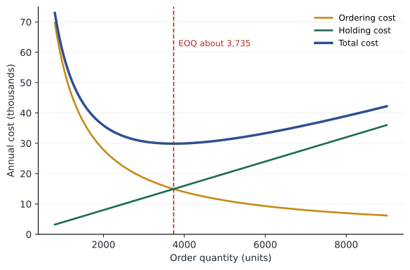
The EOQ has two lessons beyond its formula. First, the total cost curve is very flat near its minimum: ordering twice or half the optimal quantity raises total cost by only 25 per cent, and a 20 per cent error raises it by about 2 per cent. The model therefore tolerates rough estimates of S and H. Second, the optimal batch grows only with the square root of demand and setup cost. Halving the setup cost cuts the optimal batch, and therefore cycle inventory, by about 29 per cent, and cutting it to a quarter halves both. This is the economic case for the quick changeovers of lesson 5: the lean emphasis on small batches is not a rejection of the EOQ but a decision to attack its setup cost term.

Reorder points and safety stock

The EOQ says how much to order. The reorder point says when. If demand were known, a firm would order when stock fell to the demand expected during the replenishment lead time. Because demand varies, it adds safety stock to protect against higher-than-expected demand during the lead time. With average demand d per period, a lead time of L periods and a standard deviation of demand per period of sigma, the standard deviation of demand over the lead time is sigma times the square root of L, if demand in successive periods is independent. The safety stock for a chosen service level is z times that, where z is the standard normal value for the probability of not running out in a replenishment cycle, called the cycle service level.

When lead time itself varies, with standard deviation sigma-L, the second form applies, and a variable lead time can dominate the calculation: an unreliable supplier forces more safety stock than an unpredictable customer. A cycle service level of 95 per cent means a stockout in one replenishment cycle in twenty, not that 95 per cent of demand is met. The fill rate, the share of demand met from stock, is usually much higher than the cycle service level because shortages, when they happen, are often small. Managers should state which measure they mean.

In a periodic review system, stock is checked every T periods and topped up to an order-up-to level, as in most retail replenishment. The order-up-to level must cover demand over the review period plus the lead time, T + L, with safety stock based on the standard deviation over that longer interval. Longer review periods therefore need more safety stock. Fairway's stores review most grocery items daily, which keeps safety stock low; its suppliers deliver some slow-moving items only weekly, which is one reason those items run out.

import math
from statistics import NormalDist

# Cedarline's core fleece: replenished all year from one factory
D = 31000          # units a year
S = 1800           # dollars per order (factory setup, booking, administration)
c, rate = 32, 0.25 # unit cost and annual holding rate
H = c * rate
Q = math.sqrt(2 * D * S / H)
cost = lambda q: D / q * S + q / 2 * H
print(f"EOQ {Q:,.0f} units, {D / Q:.1f} orders a year, annual cost {cost(Q):,.0f} dollars")
for q in (Q / 2, 2 * Q):
    print(f"  ordering {q:,.0f}: cost {cost(q):,.0f} (+{cost(q) / cost(Q) - 1:.0%})")

d, sigma, L = D / 52, 90, 10   # weekly demand, weekly standard deviation, lead time in weeks
for csl in (0.90, 0.95, 0.99):
    z = NormalDist().inv_cdf(csl)
    ss = z * sigma * math.sqrt(L)
    print(f"Service {csl:.0%}: z {z:.2f}, safety stock {ss:,.0f}, reorder point {d * L + ss:,.0f}, holding cost {ss * H:,.0f}")

# Pooling: safety stock for one style held in 62 stores or in one place
sd_store = 6
print(f"Separate stores: {62 * sd_store} units of standard deviation; pooled: {sd_store * math.sqrt(62):.0f}")

EOQ 3,735 units, 8.3 orders a year, annual cost 29,880 dollars
  ordering 1,867: cost 37,350 (+25%)
  ordering 7,470: cost 37,350 (+25%)
Service 90%: z 1.28, safety stock 365, reorder point 6,326, holding cost 2,918
Service 95%: z 1.64, safety stock 468, reorder point 6,430, holding cost 3,745
Service 99%: z 2.33, safety stock 662, reorder point 6,624, holding cost 5,297
Separate stores: 372 units of standard deviation; pooled: 47

For the fleece, the economic order quantity is about 3,700 units, roughly eight orders a year, and ordering half or twice that amount would raise the annual ordering and holding cost by 25 per cent. With a ten-week lead time and weekly demand varying by about 90 units, a 95 per cent cycle service level needs about 470 units of safety stock, and moving to 99 per cent needs about 660, an extra 190 units that cost about 1,550 dollars a year to hold. The cost of service rises steeply at high levels because the normal distribution's tail is thin. The last line previews a point lesson 10 develops: if the same style's safety stock were held in one place rather than in 62 stores with independent demand, the variability to be covered would fall from 372 to about 47 units of standard deviation, the square-root law of pooling.

The newsvendor model

Many products cannot be reordered within the selling season. Newspapers, bakery items, fashion apparel, Christmas trees and seats on a particular flight must be stocked once, before demand is known, and anything left over is sold at a loss or thrown away. The newsvendor model sets that single order quantity. Let Cu be the cost of underage, the margin lost for each unit of demand that cannot be met, and Co the cost of overage, the loss on each unit left unsold: its cost minus whatever it can be salvaged for. The optimal quantity is the one at which the probability that demand is no greater than the quantity equals the critical ratio.

The intuition is marginal. Ordering one more unit gains Cu if demand turns out to be higher than the order and loses Co if it turns out to be lower. The firm should keep adding units until the probability of selling the last one, times Cu, equals the probability of not selling it, times Co. High-margin products with good salvage values, where Cu is large compared with Co, deserve generous stock; low-margin perishables with no salvage value deserve tight orders even at the cost of frequent stockouts. The model also shows that the order should rise above the mean forecast only when the critical ratio exceeds one-half.

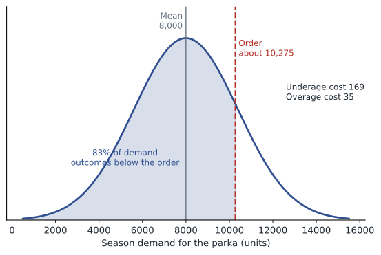
Cedarline's winter parka illustrates both sides. It sells at a full price of 289 dollars and costs 120 dollars landed. Units left at the end of the season have been sold through the outlet stores at an average of 85 dollars, so Co is 35 dollars and Cu is 169. The critical ratio is 169 / 204 = 0.83, so with demand forecast at 8,000 units with a standard deviation of 2,400, the optimal buy is about 8,000 + 0.95 × 2,400, or roughly 10,300 units. But that salvage value assumes leftover parkas can be cleared without hurting full-price sales. If clearing them through promotions in Cedarline's own stores and website trains customers to wait for discounts, as the cohort found in MBA-512, the true salvage value is lower. At an effective salvage value of 40 dollars, Co rises to 80, the critical ratio falls to 0.68, and the optimal buy falls to about 9,100. Cedarline's managers had been buying to the sales target plus a cushion, which implied a much higher ratio than either calculation supports.

The newsvendor also explains Grace's fresh departments. A loaf of in-store bread sells for 4.50 dollars, costs 1.60 and has no salvage value at the end of the day except a small donation tax benefit, so Co is about 1.60 and Cu about 2.90; the critical ratio is 0.64. A rotisserie chicken sells for 12.99, costs 7.80 and can be turned into prepared salads the next day, giving it a salvage value of about 4; Co is 3.80, Cu 5.19, and the ratio is 0.58. Fairway's store managers had been told to avoid empty shelves at all costs, which amounts to using a ratio near 0.95 for every item. Setting each item's order by its own critical ratio, with a forecast for each day of the week, is Grace's first project. Fairway's pilot in six stores cut fresh waste by about a third while reducing gaps, because orders shifted from overstocked slow sellers to understocked fast ones.