Capacity planning and waiting lines

Leo starts the seventh session with a complaint about his own company. Kestrel's customer support team handles chats and calls from retailers using its forecasting software. On average, 60 contacts arrive an hour during the business day, and an agent spends about 6 minutes on each, so the work requires six agents' worth of time. Kestrel staffs seven. Yet customers wait almost four minutes on average, and the support manager wants two more agents. Kestrel's chief executive argues that seven agents with six hours of work an hour between them are already 86 per cent busy, so the problem must be productivity. Dr. Raman tells Leo that both of them are partly right and that the arithmetic of queues explains why.

Capacity strategy

Capacity planning asks how much capacity to have, when to add it and in what increments. In the long term, it is a strategic decision about plants, distribution centres, hospitals and data centres that take years to build. In the medium term, it is about shifts, staffing, overtime and subcontracting. In the short term, it is about scheduling the capacity that exists. Three broad strategies describe how firms add capacity when demand grows. A lead strategy adds capacity ahead of demand, accepting idle capacity for a time in return for never turning customers away. A lag strategy adds capacity only after demand has arrived, keeping utilization high but losing some sales and straining service. A match strategy adds smaller increments close to the demand curve. Large, lumpy investments with economies of scale push firms toward leading or lagging; flexible capacity, such as contract manufacturers or third-party warehouses, makes matching possible.

The amount by which capacity exceeds expected demand is the capacity cushion. Firms facing uncertain demand, high costs of turning customers away or customers who will not wait need larger cushions. Electricity grids, emergency departments and fire services carry large cushions because the cost of running short is so high; a steel mill or a refinery runs close to full because idle capacity is expensive and its products can be stored. The cohort met capacity decisions under uncertainty in MBA-502 and MBA-511, where Cedarline's second distribution centre and its 18 new stores were treated as options: building in stages, and only when demand is proven, preserves the value of waiting. Dr. Raman adds an operations point. Whether the second distribution centre is needed depends not only on volume but also on how much capacity the existing building has, and lesson 3 suggested that a better layout could recover a good part of it.

Why queues form

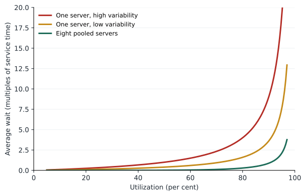
The chief executive's arithmetic treats the support desk as if contacts arrived evenly, one every minute, and took exactly six minutes each. If that were true, seven agents would never keep anyone waiting. Queues form because of variability. Contacts arrive in clumps, some take two minutes and some twenty, and when several long contacts coincide with a burst of arrivals, a queue builds that takes time to clear. Capacity that goes unused in a quiet moment cannot be saved for a busy one, because service cannot be stored. The result is that waiting depends not only on average utilization but on variability, and it rises steeply as utilization approaches 100 per cent.

A useful approximation, due to John Kingman in 1961, describes the average wait in a queue in front of a single server as the product of three terms: a variability term, a utilization term and the average processing time. The variability term is the average of the squared coefficients of variation of the times between arrivals and of the processing times, where a coefficient of variation is a standard deviation divided by its mean. The utilization term is rho divided by one minus rho. When arrivals are completely random, their coefficient of variation is 1, and when processing times are also highly variable, the variability term is about 1.

The utilization term carries the most important lesson of the chapter. At 50 per cent utilization, rho / (1 - rho) is 1; at 80 per cent, 4; at 90 per cent, 9; at 95 per cent, 19; and at 98 per cent, 49. Waiting does not rise in proportion to utilization but explodes as utilization approaches 100 per cent. A manager who pushes a busy service from 90 to 95 per cent utilization to save one staff member may double the wait. The variability term shows the other lever: halving the variability of arrivals and service, for example through appointments, standard procedures and triage that separates simple from complex cases, can cut waits as much as adding capacity.

The M/M/c queue

For many service systems, a standard model gives exact results. In queueing notation, an M/M/c system has random, or Poisson, arrivals at rate lambda, exponentially distributed service times with rate mu per server, and c identical servers drawing from a single queue. The offered load is a = lambda / mu, the number of servers' worth of work arriving, and utilization is rho = a / c, which must be below 1 for the queue to be stable. The Danish engineer Agner Krarup Erlang, who worked for the Copenhagen Telephone Company, derived the probability that an arriving customer must wait in such a system in work published between 1909 and 1917, and the formula still bears his name. It is used to staff call centres, help desks, emergency services and checkouts.

Two derived measures are commonly used. The average wait in queue, Wq, is the probability of waiting divided by the rate at which the queue empties, c times mu minus lambda. The service level, the share of customers who wait no more than a target time t, is one minus the probability of waiting times e to the power of minus (c mu minus lambda) t. Call centres often set a target such as 80 per cent of calls answered within 20 seconds. Little's law then gives the average number waiting as lambda times Wq.

import math

def erlang_c(lam, mu, c):
    a = lam / mu
    rho = a / c
    s = sum(a ** k / math.factorial(k) for k in range(c))
    top = a ** c / math.factorial(c) / (1 - rho)
    return top / (s + top)

def mmc(lam, mu, c, t):
    pw = erlang_c(lam, mu, c)
    wq = pw / (c * mu - lam)
    return pw, wq, 1 - pw * math.exp(-(c * mu - lam) * t)

lam, mu = 60, 10   # contacts per hour; each agent serves 10 an hour (6 minutes each)
print("Agents  busy   P(wait)  avg wait (min)  answered within 1 min")
for c in range(7, 11):
    pw, wq, sl = mmc(lam, mu, c, 1 / 60)
    print(f"{c:6} {lam / (c * mu):5.0%} {pw:8.1%} {wq * 60:14.2f} {sl:15.1%}")

# Pooling: two separate queues of 30 contacts an hour with 4 agents each, or one queue with 8
_, w_sep, _ = mmc(30, 10, 4, 1 / 60)
_, w_pool, _ = mmc(60, 10, 8, 1 / 60)
print(f"Separate queues: {w_sep * 60:.2f} min; one pooled queue: {w_pool * 60:.2f} min")

# Kingman's approximation for one triage nurse, 6 minutes per patient, 7 patients an hour
p, rho = 6.0, 7 * 6 / 60
for ca in (1.0, 0.6):
    wq = (ca ** 2 + 0.5 ** 2) / 2 * rho / (1 - rho) * p
    print(f"Arrival variability {ca}: average wait about {wq:.1f} minutes")

Agents  busy   P(wait)  avg wait (min)  answered within 1 min
     7   86%    61.4%           3.68           48.0%
     8   75%    35.7%           1.07           74.4%
     9   67%    19.6%           0.39           88.1%
    10   60%    10.1%           0.15           94.8%
Separate queues: 3.06 min; one pooled queue: 1.07 min
Arrival variability 1.0: average wait about 8.7 minutes
Arrival variability 0.6: average wait about 4.3 minutes

The table settles the argument at Kestrel. With seven agents, 86 per cent busy, 61 per cent of customers wait and the average wait is 3.7 minutes, matching what customers report. An eighth agent cuts the average wait to about one minute and lets about three-quarters of customers through within a minute; a ninth cuts it to under half a minute. The second agent the support manager wants adds less than the first, the usual pattern of diminishing returns. Leo's team settles on eight agents in the busiest hours and seven at quieter times, and works on the variability side as well, adding answers to the most common questions inside the software so that simple contacts never reach the queue and the remaining ones are more uniform.

Pooling

The code also shows the power of pooling. Suppose Kestrel's support team were split into two groups of four, one for Canadian and one for American customers, each receiving 30 contacts an hour. Each group would have the same utilization as a single team of eight receiving all 60 contacts, but customers would wait about three times as long on average, 3.1 minutes against 1.1. In separate queues, one group can be overwhelmed while the other has an idle agent; a pooled queue lets any free agent take the next customer. The same principle explains why banks and airports moved to a single snaking line feeding many counters, why hospitals pool operating rooms and beds across services where they can, and, in lesson 9, why holding inventory in one place requires less safety stock than holding it in many.

Pooling has limits. Pooled servers must be able to serve every customer, which requires cross-training and may lower efficiency if specialists are faster at their own work. Customers in one long line may perceive the wait as worse than in several short ones, even if it is not. And very large pooled systems can lose the personal relationship that some customers value. Hana's emergency department pools nurses across its acute and minor treatment areas during the night, when volume is low, but keeps them separate in the evening peak, when the minor area's fast flow would be disrupted by acute patients.

Managing the experience of waiting

Waiting is a psychological as well as an arithmetic problem. David Maister's 1985 essay on the psychology of waiting lines proposed principles that service firms still use: unoccupied time feels longer than occupied time; waits before service begins feel longer than waits during service; anxiety makes waits seem longer; uncertain and unexplained waits feel longer than known, explained ones; unfair waits feel longer than equitable ones; and the more valuable the service, the longer people will wait. Disney displays expected waiting times at its rides and sets them slightly above the expected value, so that most guests are pleasantly surprised. Hana's team adds a screen to the evening clinic showing the expected time to see a clinician and texts patients when they are next, so they can wait in a café rather than the waiting room.

Queue discipline, the rule for choosing who is served next, also matters. First-come, first-served is perceived as fair. Emergency departments triage by urgency, which is right clinically but must be explained so that less urgent patients understand why others go first. Priority for short jobs, such as an express checkout lane, cuts the average wait because short jobs no longer wait behind long ones. Reservations and appointments reduce arrival variability, at the cost of some flexibility for customers. Pricing can shift demand away from peaks, as with off-peak electricity rates, matinee tickets or weekday hotel rates, and revenue management, developed by airlines after deregulation, uses price to fill fixed capacity profitably.