Optimization models: calculus, constraints and linear programming

Prescriptive models answer the question 'what should we do?'. They have a common structure: decision variables that we control, an objective function that measures how good a decision is, and constraints that limit the choices. This lesson builds optimization models for the transit agency and the fisheries office. We start with unconstrained problems solved by calculus, which lead to the famous square-root law for bus headways, move to equality constraints and Lagrange multipliers, and then to linear programming, where the constraints are inequalities and the optimum lies at a corner of the feasible region. Throughout, the most useful output is often not the optimal decision itself but the sensitivity of the optimum to the constraints, measured by shadow prices.

The anatomy of an optimization model

An optimization model has the form: choose decision variables \(x = (x_1, \dots, x_n)\) to maximize or minimize an objective \(f(x)\) subject to constraints \(g_j(x) \le b_j\) and \(h_k(x) = c_k\). Formulating such a model is a modelling task like any other. The decision variables must be things the decision maker can actually set; the objective must reflect what the decision maker cares about, which often means combining several goals, such as cost and service quality, into one measure with explicit weights; and the constraints must capture the real limits, such as budgets, capacities and regulations.

The choice of objective deserves particular care. Maximizing the total catch, the total profit and the long-term health of the fish stock lead to different policies. A model cannot tell us which goal is right; it can tell us precisely what each goal implies and what trade-offs exist between them. Presenting those trade-offs to decision makers is often the most valuable thing a modeller can do.

Unconstrained optimization: the square-root law

How often should buses run on Route 9? Running more buses costs money; running fewer makes passengers wait. Let the headway be \(h\) hours. A round trip takes \(T\) hours, so the route needs \(\frac{T}{h}\) buses, each costing \(c_b\) dollars per hour to operate. Passengers arrive at random at a rate \(\lambda\) per hour and, with regular buses, wait on average \(\frac{h}{2}\). If the agency values passenger time at \(c_w\) dollars per hour, the total cost per hour is \[C(h) = \frac{c_bT}{h} + \frac{\lambda c_wh}{2}.\]

The first term decreases with \(h\) and the second increases, so there is a balance. Setting \(C^\prime(h) = -\frac{c_bT}{h^2} + \frac{\lambda c_w}{2} = 0\) gives \[h^* = \sqrt{\frac{2c_bT}{\lambda c_w}}.\] Since \(C^{\prime\prime}(h) = \frac{2c_bT}{h^3} > 0\), this is a minimum. At the optimum the two costs are equal, a common feature of problems with this structure. The optimal headway grows only as the square root of the operating cost and falls as the square root of demand: quadrupling ridership should halve the headway, not quarter it. The same square-root law appears in the classical economic order quantity model of inventory, where ordering costs are balanced against storage costs.

The model also explains why off-peak service is less frequent. At 150 passengers per hour, a quarter of the rush-hour demand, the optimal headway doubles to 24 minutes. A refinement accounts for bunching from lesson 4, which makes the average wait longer than \(\frac{h}{2}\) when headways are irregular; the formula becomes \(\frac{h}{2}(1 + \frac{\sigma^2}{h^2})\), where \(\sigma\) is the standard deviation of headways, and reliability then has a measurable dollar value.

Equality constraints and Lagrange multipliers

Now suppose the agency has a fixed fleet of \(N\) buses to divide between routes. Route \(i\) has round-trip time \(T_i\) and demand \(\lambda_i\); assigning \(n_i\) buses gives headway \(\frac{T_i}{n_i}\) and total waiting time per hour \(\frac{\lambda_iT_i}{2n_i}\). To minimize total waiting subject to \(\sum n_i = N\), treat the \(n_i\) as continuous and form the Lagrangian \[\mathcal{L} = \sum_i \frac{\lambda_iT_i}{2n_i} + \mu\Big(\sum_i n_i - N\Big).\] Setting \(\frac{\partial \mathcal{L}}{\partial n_i} = -\frac{\lambda_iT_i}{2n_i^2} + \mu = 0\) gives \(n_i = \sqrt{\frac{\lambda_iT_i}{2\mu}}\), so \[n_i \propto \sqrt{\lambda_iT_i}.\] Buses should be allocated in proportion to the square root of demand times trip length, not in proportion to demand. Busy routes get more buses, but less than proportionally more, because the benefit of an extra bus diminishes as the headway shrinks.

The multiplier \(\mu\) has an important meaning. At the optimum, \(\mu\) equals the rate at which the minimum total waiting time decreases per extra bus added to the fleet. In general, the Lagrange multiplier of a constraint is the sensitivity of the optimal value to the constraint's right-hand side. Economists call it a shadow price: it tells the decision maker how much it would be worth to relax the constraint by one unit, and so whether buying another bus, hiring another driver or raising the budget is worthwhile.

Linear programming

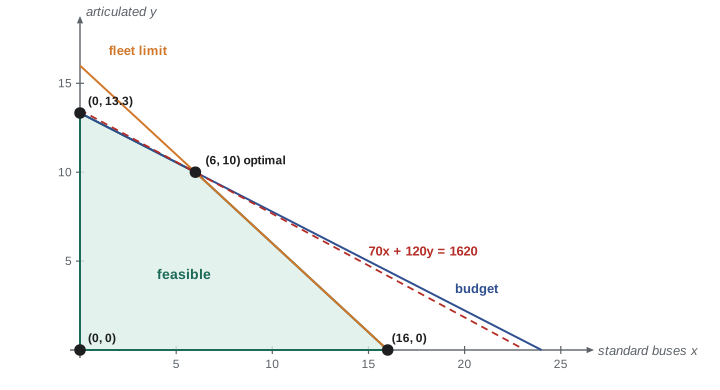
Many practical problems have linear objectives and linear inequality constraints. The transit agency is buying new buses with a capital budget of 12 million dollars. Standard buses cost 0.5 million and carry 70 passengers; articulated buses cost 0.9 million and carry 120. The union contract and depot space allow at most 16 new buses in total, because each needs a driver. How many of each should be bought to maximize total capacity?

Let \(x\) and \(y\) be the numbers of standard and articulated buses. The model is \[\text{maximize } 70x + 120y \quad \text{subject to} \quad 0.5x + 0.9y \le 12, \quad x + y \le 16, \quad x, y \ge 0.\] The constraints define a convex polygon, the feasible region. The objective's level sets are parallel lines, and moving them in the direction of increase, the last point of the region they touch is the optimum. Since the objective is linear, that point is a corner, or vertex, of the polygon, or possibly a whole edge.

Theorem 8.1 (fundamental theorem of linear programming). If a linear program has an optimal solution and its feasible region has at least one vertex, then some vertex is optimal. The theorem reduces an infinite search to a finite one. For two variables we can list the vertices by hand; for thousands of variables, the simplex method, invented by George Dantzig in 1947, moves from vertex to vertex along edges, improving the objective at each step, and is among the most widely used algorithms in the world.

Shadow prices and sensitivity

At the optimum both constraints are binding, holding with equality. Their shadow prices tell the agency what an extra unit of each resource would be worth. Increasing the budget by 1 million while keeping 16 buses moves the vertex to \(x + y = 16\), \(0.5x + 0.9y = 13\), giving \(y = 12.5\), \(x = 3.5\) and capacity 1745: the budget's shadow price is 125 passengers per million dollars. Similarly an extra driver is worth \(7.5\) passengers. These values solve the dual linear program, \(0.5u + v = 70\), \(0.9u + v = 120\), whose solution \((u, v) = (125, 7.5)\) assigns a value to each resource so that each bus type's capacity exactly equals the value of the resources it uses.

Shadow prices are valid only over a range. If the budget grows past 14.4 million, the vertex \((x, y)\) reaches \(x = 0\) and the structure of the solution changes: the agency would buy only articulated buses and the driver limit alone would bind. Linear programming software reports these ranges, and they are as important as the optimum itself, since a decision maker wants to know how robust a recommendation is to changes in prices, budgets and demand.

# Vertex enumeration for a small linear program, in exact arithmetic
from fractions import Fraction as F
from itertools import combinations

def solve_lp(c, A, b):
    """maximize c.x subject to A x <= b and x >= 0, for two variables"""
    rows = [(a, bi) for a, bi in zip(A, b)] + [((F(-1), F(0)), F(0)), ((F(0), F(-1)), F(0))]
    best = None
    for (a1, b1), (a2, b2) in combinations(rows, 2):
        det = a1[0] * a2[1] - a1[1] * a2[0]
        if det == 0:
            continue
        x = ((b1 * a2[1] - a1[1] * b2) / det, (a1[0] * b2 - b1 * a2[0]) / det)
        if all(a[0] * x[0] + a[1] * x[1] <= bi for a, bi in rows):
            val = c[0] * x[0] + c[1] * x[1]
            if best is None or val > best[0]:
                best = (val, x)
    return best

c = (F(70), F(120))
A = [(F(1, 2), F(9, 10)), (F(1), F(1))]
for budget in [12, 13, 14, 15]:
    val, x = solve_lp(c, A, [F(budget), F(16)])
    print(f"budget {budget}M: buy {float(x[0]):4.1f} standard, {float(x[1]):5.2f} articulated, capacity {float(val):7.1f}")

budget 12M: buy  6.0 standard, 10.00 articulated, capacity  1620.0
budget 13M: buy  3.5 standard, 12.50 articulated, capacity  1745.0
budget 14M: buy  1.0 standard, 15.00 articulated, capacity  1870.0
budget 15M: buy  0.0 standard, 16.00 articulated, capacity  1920.0

The output shows the shadow price of 125 passengers per million between 12 and 14 million. At 15 million the solution has changed structure: all 16 buses are articulated and the budget is no longer binding, so a further million adds nothing. Practical problems of this kind, scheduling buses and drivers across a whole network, assigning aircraft to routes or blending animal feed at least cost, have thousands of variables and are solved routinely by commercial and open-source solvers, often with the extra requirement that variables be integers.

Optimizing the fishery

Return to the constant-effort fishery of lesson 5, now with economics. Suppose fish sell for \(p\) dollars each and effort costs \(c\) dollars per unit per year. At the sustained equilibrium the annual profit is \[\Pi(E) = pEK\Big(1 - \frac{E}{r}\Big) - cE.\] Setting \(\Pi^\prime(E) = pK(1 - \frac{2E}{r}) - c = 0\) gives \[E^* = \frac{r}{2}\Big(1 - \frac{c}{pK}\Big),\] which is less than the MSY effort \(\frac{r}{2}\). Taking cost into account, the profit-maximizing fishery fishes less and keeps a larger stock than the MSY fishery, because the last few fish of the maximum yield cost more to catch than they are worth.

Without regulation the outcome is different. Under open access, new boats enter as long as fishing is profitable, so effort grows until profit falls to zero: \(pK(1 - \frac{E}{r}) = c\), or \(E_\infty = r(1 - \frac{c}{pK})\), exactly twice the optimal effort. This is the Gordon–Schaefer model of 1954, the first mathematical account of what was later called the tragedy of the commons: individually rational decisions lead to overfishing and dissipate all the profit the resource could generate. The model is the starting point for the economics of licence limits, individual transferable quotas and marine reserves.