Compartment models and the spread of epidemics

A compartment model divides a population into groups, or compartments, according to their state, and describes the flows of individuals between them. The most famous example is the SIR model of an epidemic, introduced by William Kermack and Anderson McKendrick in 1927. This lesson derives the model, uses the phase plane and the scaled form of lesson 3 to find its threshold, peak and final size exactly, and then applies it to the city public health unit's questions about the influenza season: how many people will be ill at the peak, when the peak will come, and what a week of school closures would change.

Compartments and flows

Divide a city of \(P\) people into three compartments: susceptible \(S\), who can catch the disease; infectious \(I\), who have it and can pass it on; and removed \(R\), who have recovered with immunity. The model rests on four assumptions. The population is closed, with no births, deaths from other causes or migration over the season. It is well mixed, so every infectious person is equally likely to meet every susceptible one. New infections occur at a rate proportional to the number of contacts between susceptible and infectious people, \(\beta SI\). Infectious people recover at a constant per capita rate \(\gamma\), so the infectious period is exponentially distributed with mean \(\frac{1}{\gamma}\).

These assumptions translate directly into equations, one per compartment, by balancing inflow and outflow: \[\frac{dS}{dt} = -\beta SI, \qquad \frac{dI}{dt} = \beta SI - \gamma I, \qquad \frac{dR}{dt} = \gamma I.\] Adding the three equations gives \(\frac{d}{dt}(S + I + R) = 0\), so the total \(P\) is conserved, as it must be in a closed population. The standard way to draw the model is a flow diagram with a box for each compartment and an arrow for each flow, labelled with its rate.

Some modellers write the infection term as \(\frac{\beta SI}{P}\) instead, so that \(\beta\) is the number of effective contacts per infectious person per day. The two forms are equivalent for a fixed population and differ only in the units of \(\beta\). In what follows, after scaling, all that matters is the dimensionless number \(R_0 = \frac{\beta P}{\gamma}\) found in lesson 3.

The epidemic threshold

In the scaled variables \(s = \frac{S}{P}\), \(i = \frac{I}{P}\) and \(\tau = \gamma t\), the model is \[s^\prime = -R_0si, \qquad i^\prime = (R_0s - 1)i.\] The second equation gives the threshold immediately. The number infectious increases when \(R_0s > 1\) and decreases when \(R_0s < 1\). At the start of an outbreak almost everyone is susceptible, \(s \approx 1\), so an outbreak can grow only if \(R_0 > 1\). Each case must, on average, cause more than one new case.

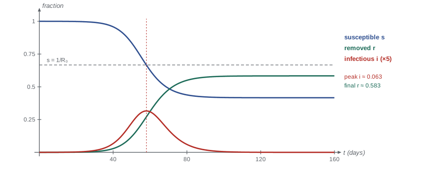
The quantity \(R_t = R_0s(t)\) is the effective reproduction number, the average number of new cases caused by one case at time \(t\). It falls as susceptible people are infected. The epidemic peaks when \(R_t = 1\), that is when \(s = \frac{1}{R_0}\), and declines afterward, not because the disease has disappeared but because there are too few susceptible people left to sustain growth. If a fraction \(1 - \frac{1}{R_0}\) of the population is immune before the outbreak, for example by vaccination, then \(R_0s(0) \le 1\) and no outbreak can grow. This is the herd immunity threshold: about 33% for \(R_0 = 1.5\), typical of seasonal influenza, and about 93% for \(R_0 = 15\), typical of measles.

Early in an outbreak, with \(s \approx 1\), the infectious number grows exponentially as \(i \approx i_0e^{(R_0 - 1)\tau}\), or in dimensional time at the rate \(\rho = \gamma(R_0 - 1)\) per day. This links \(R_0\) to the observed early doubling time \(T_d = \frac{\ln 2}{\rho}\), and is how \(R_0\) is usually estimated at the start of a new epidemic: measure the doubling time, estimate the infectious period, and solve for \(R_0 = 1 + \frac{\ln 2}{\gamma T_d}\).

Peak and final size

The phase plane of \((s, i)\) gives exact results. Dividing the equations, \[\frac{di}{ds} = \frac{(R_0s - 1)i}{-R_0si} = -1 + \frac{1}{R_0s},\] which integrates to \[i + s - \frac{1}{R_0}\ln s = \text{constant} = i_0 + s_0 - \frac{1}{R_0}\ln s_0.\] Every trajectory is a level curve of this conserved quantity.

The peak occurs at \(s = \frac{1}{R_0}\). With \(i_0 \approx 0\) and \(s_0 \approx 1\), the peak fraction infectious is \[i_{\max} = 1 - \frac{1 + \ln R_0}{R_0}.\] The final size is the fraction \(z\) of the population ever infected. At the end \(i = 0\) and \(s = 1 - z\), so \(1 - z - \frac{1}{R_0}\ln(1 - z) = 1\), which rearranges to the final size equation \[1 - z = e^{-R_0z}.\] For \(R_0 > 1\) this has exactly one root in \((0, 1)\), found numerically. The epidemic does not infect everyone: some susceptible people escape because the infectious population dies out first.

Interventions

The public health unit asks whether closing schools for a week would help. In the model, a closure reduces contacts and hence \(\beta\) for its duration. Its effect depends strongly on timing. A closure long before the peak delays the epidemic but barely changes its size once contacts resume, because the susceptible pool is still almost full. A closure in the days just before the peak, while many people are infectious and the susceptible pool is close to the threshold, removes transmission when it matters most: it lowers the peak and reduces the final size somewhat, because the epidemic ends closer to the herd immunity threshold with less overshoot. A closure after the peak cannot lower the peak at all, although one shortly after it still trims the overshoot.

Overshoot is the difference between the final size and the herd immunity threshold, \(z - (1 - \frac{1}{R_0})\). For \(R_0 = 1.5\) it is about \(0.583 - 0.333 = 0.25\): the epidemic infects a quarter of the population more than is needed to stop it, because infections continue after the peak. Well-timed interventions reduce overshoot. The program below compares closures at different times.

# SIR for a city of 500,000: effect of a one-week closure that cuts transmission by 25%
P, gamma, R0 = 500_000, 1 / 3, 1.5
beta = R0 * gamma / P

def season(close_start=None, length=7, cut=0.25, days=240, dt=0.01):
    S, I, R, t = P - 10.0, 10.0, 0.0, 0.0
    peak, t_peak = I, 0.0
    for _ in range(int(days / dt)):
        b = beta * (1 - cut) if close_start is not None and close_start <= t < close_start + length else beta
        new_inf, rec = b * S * I * dt, gamma * I * dt
        S, I, R, t = S - new_inf, I + new_inf - rec, R + rec, t + dt
        if I > peak:
            peak, t_peak = I, t
    return peak, t_peak, R + I

base = season()
print(f"no closure:      peak {base[0]:7,.0f} on day {base[1]:5.1f}, total infected {base[2]:8,.0f}")
for start in [20, 40, 50, 55, 62, 75]:
    pk, tp, tot = season(start)
    print(f"closure day {start:3d}: peak {pk:7,.0f} on day {tp:5.1f}, total infected {tot:8,.0f}")

no closure:      peak  31,533 on day  57.9, total infected  291,468
closure day  20: peak  31,345 on day  63.2, total infected  291,153
closure day  40: peak  27,225 on day  64.2, total infected  283,908
closure day  50: peak  22,605 on day  50.0, total infected  268,590
closure day  55: peak  30,174 on day  55.0, total infected  263,850
closure day  62: peak  31,533 on day  57.9, total infected  269,565
closure day  75: peak  31,533 on day  57.9, total infected  285,230

The output shows the pattern. Without intervention the peak of about 31,500 infectious people comes near day 58. A closure starting on day 20 only delays the epidemic slightly. A closure covering the week before the peak, starting on day 50, cuts the peak by about 28%, to roughly 22,600, and reduces the total by about 23,000. A closure starting on day 55 lowers the peak less but trims the total the most, by reducing overshoot. Closures starting after the peak leave the peak unchanged, and one starting as late as day 75 achieves little. For hospital planning the peak matters more than the total, and the model tells the health unit that the timing of the closure is as important as its strength, which in turn means that good surveillance data, showing where the epidemic is on its curve, are essential.

Extending the model

The SIR model is a starting point. Influenza has a latent period of a day or two in which people are infected but not yet infectious; adding an exposed compartment \(E\) gives the SEIR model, \[S^\prime = -\beta SI, \quad E^\prime = \beta SI - \sigma E, \quad I^\prime = \sigma E - \gamma I, \quad R^\prime = \gamma I,\] with mean latent period \(\frac{1}{\sigma}\). Its \(R_0\) is still \(\frac{\beta P}{\gamma}\), and its final size equation is the same, but its epidemic is slower. Diseases in which immunity wanes, such as common colds, need a flow from \(R\) back to \(S\), giving the SIRS model, which can settle to an endemic equilibrium with the disease always present.

Vaccination before the season moves a fraction \(p\) of the population directly from \(S\) to \(R\), so \(s_0 = 1 - p\) and the effective reproduction number at the start is \(R_0(1 - p)\). Heterogeneity matters too: children mix more than adults, so an age-structured model with separate compartments for each age group and a contact matrix between them gives a better description, and shows why vaccinating schoolchildren, who drive transmission, can protect older people more than vaccinating older people directly. The reproduction number of such a model is the dominant eigenvalue of a next-generation matrix, a generalization of the scalar \(R_0\).

Finally, randomness matters at the start. With only a handful of cases, chance determines whether the outbreak takes off. In a stochastic version of the model, a single case starts a major outbreak with probability approximately \(1 - \frac{1}{R_0}\), only one in three for \(R_0 = 1.5\). Lesson 9 develops the tools for such calculations.

Compartment models elsewhere

The same structure of boxes and flows appears throughout applied mathematics. Pharmacokinetic models track a drug moving from the gut to the blood to the tissues. Models of rumour spreading and the adoption of new technology have the form of SIR. Models of pollutants in a chain of lakes have one compartment per lake, with outflow from each feeding the next. In each case, writing the balance law for each compartment, inflow minus outflow, produces the equations, and the phase plane and threshold analysis of this lesson apply.