Continuous population models: logistic growth and harvesting

This lesson studies the continuous-time model of the Larch Lake fishery in detail. We derive the logistic equation, solve it exactly, and then introduce the phase line, a qualitative tool that finds equilibria and their stability without solving anything. Applied to harvesting, the phase line explains the threshold seen in the simulation of lesson 1, identifies the maximum sustainable yield, and shows why a policy based on a fixed quota is far more dangerous than one based on fixed fishing effort.

From exponential to logistic growth

If each fish produces offspring and dies at constant per capita rates \(b\) and \(m\), the population changes at the rate \(\frac{dN}{dt} = (b - m)N = rN\), with solution \(N(t) = N_0e^{rt}\). Exponential growth is a good description of a small population with abundant resources, such as walleye restocked into a lake after a closure. It cannot last: at 30% a year, 1000 fish would become more than a billion in 50 years.

The simplest correction assumes that the per capita growth rate declines linearly with population size, from \(r\) when the population is small to zero at the carrying capacity \(K\): \[\frac{1}{N}\frac{dN}{dt} = r\Big(1 - \frac{N}{K}\Big).\] This is the logistic equation, introduced by Pierre-François Verhulst in 1838. The linear decline is an assumption, not a law; it summarizes competition for food and spawning habitat in a single term. Its virtues are that it has the right qualitative behaviour, it has only two parameters, and both have clear meanings that can be estimated from data.

Solving the logistic equation

The logistic equation is separable. In scaled form \(x = \frac{N}{K}\), \(\tau = rt\), it reads \(\frac{dx}{d\tau} = x(1 - x)\). Separating and using partial fractions, \[\int \Big(\frac{1}{x} + \frac{1}{1 - x}\Big)dx = \int d\tau, \qquad \ln\frac{x}{1 - x} = \tau + c.\] Solving for \(x\) with \(x(0) = x_0\) gives \[x(\tau) = \frac{x_0}{x_0 + (1 - x_0)e^{-\tau}}, \qquad N(t) = \frac{KN_0}{N_0 + (K - N_0)e^{-rt}}.\]

Every solution with \(N_0 > 0\) tends to \(K\) as \(t \to \infty\). Solutions starting below \(\frac{K}{2}\) have an S-shaped graph with an inflection point at \(N = \frac{K}{2}\), where the growth rate \(\frac{dN}{dt}\) is largest; solutions starting above \(K\) decrease toward it. The time for a small population to grow from 10% to 90% of \(K\) is \(\frac{2\ln 9}{r} \approx \frac{4.4}{r}\), about 15 years for Larch Lake.

The phase line

For an autonomous equation \(\frac{dx}{dt} = f(x)\), much can be learned without solving. An equilibrium is a value \(x^*\) with \(f(x^*) = 0\). Between equilibria, \(f\) has constant sign, so \(x\) increases where \(f > 0\) and decreases where \(f < 0\). Drawing the \(x\) axis with arrows showing the direction of motion gives the phase line. Solutions cannot cross equilibria, by uniqueness of solutions, so every solution moves monotonically toward an equilibrium or to infinity.

Theorem 5.1 (linear stability for autonomous equations). If \(f\) is continuously differentiable and \(f(x^*) = 0\), then \(x^*\) is asymptotically stable if \(f^\prime(x^*) < 0\) and unstable if \(f^\prime(x^*) > 0\). Near the equilibrium, \(y = x - x^*\) satisfies \(y^\prime \approx f^\prime(x^*)y\), so perturbations decay or grow like \(e^{f^\prime(x^*)t}\).

Compare Theorem 4.1 for maps, where the condition was \(|F^\prime(x^*)| < 1\). For differential equations it is \(f^\prime(x^*) < 0\). The reason for the difference is that the perturbation of a map is multiplied by \(F^\prime\) at each step, while that of a differential equation grows at the continuous rate \(f^\prime\). For the logistic equation \(f(x) = x(1 - x)\), \(f^\prime(0) = 1 > 0\) and \(f^\prime(1) = -1 < 0\), so extinction is unstable and the carrying capacity is stable, for every \(r > 0\). The continuous logistic model can never oscillate or become chaotic, in sharp contrast with the Ricker map.

Constant-quota harvesting

Now add a catch of \(H\) fish per year. In scaled form, from lesson 3, \[\frac{dx}{d\tau} = x(1 - x) - h, \qquad h = \frac{H}{rK}.\] The equilibria are where the growth curve \(x(1 - x)\) meets the horizontal line at height \(h\): \[x_\pm = \frac{1}{2}\Big(1 \pm \sqrt{1 - 4h}\Big).\] For \(h < \frac{1}{4}\) there are two. Since \(f^\prime(x) = 1 - 2x\), the upper equilibrium \(x_+ > \frac{1}{2}\) has \(f^\prime < 0\) and is stable, while the lower one \(x_- < \frac{1}{2}\) is unstable. The lower equilibrium is a threshold: a population pushed below it, by a bad spawning year or an overestimated stock, declines to extinction even though the quota is unchanged.

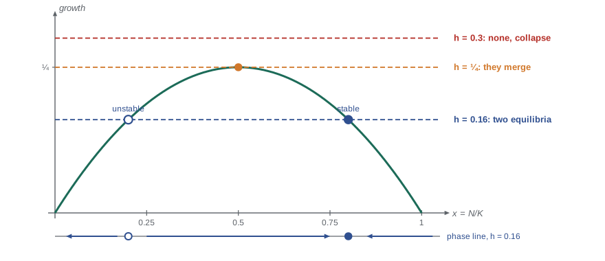
As \(h\) increases, the two equilibria move toward each other, collide at \(x = \frac{1}{2}\) when \(h = \frac{1}{4}\), and disappear. For \(h > \frac{1}{4}\) there is no equilibrium and \(\frac{dx}{d\tau} < 0\) everywhere: the population collapses from any starting value. This collision and disappearance of a stable and an unstable equilibrium is called a saddle-node bifurcation, and it is the mathematical form of a tipping point. A small increase in the quota past the critical value causes a qualitative change, from a sustainable fishery to extinction, and reducing the quota again afterward does not restore the fish, because the population has already fallen below the threshold.

The critical catch \(h = \frac{1}{4}\), or \(H = \frac{rK}{4}\), is the maximum sustainable yield (MSY). It is achieved by keeping the population at \(\frac{K}{2}\), where natural growth is fastest. For Larch Lake, MSY is 3000 fish per year at a stock of 20,000. The concept dominated fisheries management in the twentieth century, and its weaknesses, which this model already reveals, contributed to several famous collapses.

Constant-effort harvesting

An alternative policy limits fishing effort, such as the number of licences or the length of the season, rather than the catch. If each unit of effort catches a fixed fraction of the fish present, the catch is proportional to the stock: \(H = EN\), with \(E\) in 1/year. The model becomes \[\frac{dN}{dt} = rN\Big(1 - \frac{N}{K}\Big) - EN.\] For \(E < r\) the positive equilibrium is \(N^* = K(1 - \frac{E}{r})\), with \(f^\prime(N^*) = E - r < 0\), so it is stable. The sustained yield is \[Y(E) = EN^* = EK\Big(1 - \frac{E}{r}\Big),\] which is maximized at \(E = \frac{r}{2}\), giving the same maximum \(\frac{rK}{4}\) at the same stock \(\frac{K}{2}\).

The two policies have the same best case but very different failure modes. Under constant effort there is no threshold and no bifurcation as long as \(E < r\): the equilibrium moves smoothly as parameters change, and if the stock falls, the catch falls with it, automatically reducing the pressure. If \(r\) is overestimated by 10% and effort is set at \(\frac{r}{2}\) of the estimate, the true equilibrium is \(K(1 - \frac{0.15}{0.27}) \approx 0.44K\) and the yield is only about 1% below the true maximum. The comparison is a lesson about robustness: a prescriptive model should recommend policies that perform well even when the model's parameters are wrong.

# Compare a fixed quota with fixed effort when the growth rate is overestimated.
K, r_est, r_true = 40000.0, 0.30, 0.27
H_quota = r_est * K / 4          # MSY quota from the estimate
E_effort = r_est / 2             # MSY effort from the estimate

def run(policy, years=80, dt=0.01, N=20000.0):
    t, catch = 0.0, 0.0
    for _ in range(int(years / dt)):
        H = H_quota if policy == "quota" else E_effort * N
        H = min(H, N / dt)                    # cannot catch more fish than exist
        N += dt * (r_true * N * (1 - N / K) - H)
        t += dt
        catch += H * dt
        if N < 1:
            return f"stock collapsed in year {t:.0f}; total catch {catch:,.0f}"
    return f"stock {N:,.0f} after {years} years; annual catch now {H:,.0f}"

print("quota :", run("quota"))
print("effort:", run("effort"))
print("true MSY:", f"{r_true * K / 4:,.0f} fish/year")

quota : stock collapsed in year 28; total catch 83,304
effort: stock 17,778 after 80 years; annual catch now 2,667
true MSY: 2,700 fish/year

The simulation confirms the analysis. The quota policy keeps taking 3000 fish a year until the stock is exhausted. The effort policy settles at a stock near 17,800 with an annual catch near 2670, close to the true maximum of 2700. Real fisheries management now uses precautionary reference points well below MSY, harvest control rules that cut the catch when surveys show the stock falling, and explicit allowance for uncertainty, all of which can be studied with extensions of this model.

Other growth laws

The logistic law is one choice among many. The Gompertz model \(\frac{dN}{dt} = rN\ln\frac{K}{N}\) is used for tumour growth and some fish populations, and grows fastest at \(\frac{K}{e}\) rather than \(\frac{K}{2}\). Some species suffer from an Allee effect: at low density individuals have trouble finding mates or defending against predators, so per capita growth is reduced. A simple model is \[\frac{dN}{dt} = rN\Big(\frac{N}{A} - 1\Big)\Big(1 - \frac{N}{K}\Big), \qquad 0 < A < K,\] which has an unstable equilibrium at the Allee threshold \(A\) even without harvesting. Populations of this kind can collapse after a period of overfishing even if fishing stops, because they have been pushed below \(A\). The phase line analysis of each model takes a few minutes and shows immediately which conclusions depend on the choice of growth law.

Interpreting the model for Larch Lake

For the fisheries office, the model's lessons can be summarized in plain language. The lake can sustain at most about 3000 walleye a year, and only if the stock is held near 20,000. Because the growth rate is uncertain, a quota at that level risks collapse; a policy that limits effort, or a quota reduced automatically when surveys show the stock falling below a trigger level, gives nearly the same catch with far less risk. These conclusions follow from a model with two parameters, and the analysis also tells us which further data would be most valuable: a better estimate of \(r\), which lesson 10 obtains by fitting the model to survey counts.