The modelling cycle: questions, assumptions and variables

A mathematical model is a description of part of the world in the language of mathematics, built to answer a question. This first lesson sets out what models are for, how they are built and tested, and the vocabulary used throughout the course. It also introduces the three case studies that return in almost every lesson: the walleye fishery on Larch Lake, an influenza season in a city of half a million people, and a busy suburban bus route. By the end you should be able to take a vague practical question and turn it into a precise mathematical problem with named variables, stated assumptions and a plan for checking the answer.

What a model is for

Every useful model starts with a question, not with an equation. The fisheries office responsible for Larch Lake does not ask for 'a model of walleye'. It asks how many fish anglers can take each year without the population collapsing. The public health unit asks how many hospital beds will be needed at the peak of the influenza season, and whether closing schools for a week would lower that peak. The transit agency asks why buses on Route 9 arrive in bunches and whether holding them at a timing point would help. Each question tells us what output the model must produce, how accurate it needs to be and what decisions it will inform.

Models are always simplifications. A model of the lake that tracked every fish, every insect and every ripple would be as complicated as the lake and no easier to understand. The skill of modelling is choosing what to leave out. The statistician George Box put it in a phrase that every modeller quotes: all models are wrong, but some are useful. A model is useful when it captures the mechanisms that drive the answer to the question while ignoring the details that do not.

It helps to distinguish three purposes. A model can be explanatory, showing which mechanisms produce an observed pattern; predictive, forecasting what will happen under stated conditions; or prescriptive, recommending the best decision among alternatives. The same equations can serve all three, but the standard of evidence differs. An explanatory model must reproduce the qualitative pattern; a predictive one must be checked against data it was not fitted to; a prescriptive one must also be robust, giving good decisions even when its parameters are somewhat wrong.

The modelling cycle

Modelling is iterative. Textbooks and practitioners describe it as a cycle with six stages, which we will use as a checklist throughout the course.

First, state the question precisely, including what will be measured and what will be decided. Second, list the assumptions: what is included, what is ignored and what is treated as constant. Third, formulate the model: name the variables and parameters, give their units, and write the relations between them as equations, inequalities or probability rules. Fourth, solve or analyse the model, by exact methods where possible and by numerical computation otherwise. Fifth, interpret the results in the language of the original question, with units and with an honest statement of uncertainty. Sixth, validate: compare the predictions with data and with common sense, and decide whether the model is good enough or whether the assumptions must be revised, which sends us back round the cycle.

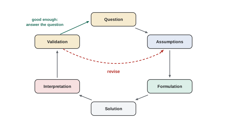
The arrow from validation back to the assumptions is the most important one in the diagram. A first model is almost never the last. It is common to start with the simplest model that could possibly answer the question, find where it fails, and add exactly the feature that repairs the failure. This incremental approach keeps the model understandable, because each feature is there for a reason that can be explained to the people who will use the answer.

Variables, parameters and units

A model distinguishes several kinds of quantity. Independent variables are the quantities we vary freely, most often time \(t\) and sometimes position \(x\). Dependent variables, or state variables, are the quantities the model predicts, such as the number of walleye \(N(t)\) or the number of people infected \(I(t)\). Parameters are quantities held fixed during a single run of the model but which may differ between situations, such as the intrinsic growth rate \(r\) of the fish population or the average number of contacts per day. Inputs or controls are quantities chosen by a decision maker, such as the annual catch limit \(H\).

Every quantity in a model should be given units, and every equation must be dimensionally consistent: both sides must have the same units. A growth rate \(r\) in the equation \(\frac{dN}{dt} = rN\) must have units of 1/year if \(N\) is a number of fish and \(t\) is in years, because the left side has units of fish per year. Checking units is the cheapest error test in all of applied mathematics, and lesson 2 shows that units carry far more information than that, often enough to determine the form of an answer before any equation is solved.

Kinds of models

Models can be classified along several independent axes, and choosing the right point on each axis is part of formulation.

Deterministic or stochastic. A deterministic model gives a single output for given inputs; a stochastic model includes randomness and produces a distribution of outputs. A deterministic model of influenza predicts one epidemic curve; a stochastic one predicts a spread of possible curves, including the possibility that the outbreak dies out early by chance. Stochastic effects matter most when numbers are small, at the start of an outbreak or for a rare species.

Discrete or continuous in time. A discrete-time model updates the state once per time step, such as once per breeding season, and is written as a difference equation \(N_{t+1} = F(N_t)\). A continuous-time model describes rates of change and is written as a differential equation. Fish that spawn once a year are naturally described in discrete time; bacteria that divide around the clock, in continuous time. Lessons 4 and 5 compare the two and show that they can behave very differently.

Lumped or distributed. A lumped model treats each variable as a single number for the whole system; a distributed model lets variables depend on position, leading to partial differential equations. A lumped model of the lake has one walleye population; a distributed one would track density across bays. Lesson 11 introduces distributed models of diffusion and traffic.

Mechanistic or empirical. A mechanistic model is derived from assumptions about how the system works, such as rates of birth, infection or flow. An empirical model is a formula chosen because it fits data, such as a straight line or a power law. Mechanistic models usually extrapolate better, because their structure reflects the causes; empirical models are often more accurate within the range of the data. Most real models mix the two, with mechanistic structure and parameters estimated from data, as in lesson 10.

Building a model from a word problem: the bus route

Route 9 runs every 10 minutes at rush hour. Passengers complain that they often wait 20 minutes and then two buses arrive together. A simple mechanism explains this. Suppose one bus falls slightly behind schedule. More passengers have accumulated at each stop, so boarding takes longer and the bus falls further behind. The bus behind it finds fewer passengers, boards quickly and catches up. The gap between them is unstable.

To capture this mechanism we need only a few quantities: the headway \(h_k\), the time gap between bus \(k\) and the bus ahead of it at a given stop; the passenger arrival rate \(\lambda\) passengers per minute; and the boarding time \(b\) minutes per passenger. If a bus arrives with headway \(h\), about \(\lambda h\) passengers are waiting and the dwell time is \(b\lambda h\). The dimensionless product \(\beta = b\lambda\) measures how strongly dwell time depends on headway. In lesson 4 we turn this into a difference equation and show that headway deviations grow from stop to stop by a factor that depends on \(\beta\), so that bunching is a predictable consequence of the mechanism, not bad luck.

This back-of-the-envelope model already gives a testable prediction: bunching should be worse on routes with many busy stops and slow boarding, and better where fares are paid before boarding, which lowers \(b\). Transit agencies have confirmed both effects. The model also suggests a remedy, holding early buses at a timing point, whose cost and benefit can be computed once the model is made precise.

Solving models: exact, numerical and qualitative

Once formulated, a model must be analysed. There are three complementary approaches. Exact solutions in closed form are the most informative when they exist, because they show how the answer depends on every parameter at once. Numerical solutions compute the answer for particular parameter values and are available for almost any model. Qualitative analysis finds properties of the solutions without computing them: equilibria, their stability, long-term behaviour, and thresholds at which the behaviour changes. The best modelling combines all three, using qualitative analysis to know what to expect and numerical work to check and extend it.

For the influenza model of lesson 7 there is no closed-form solution for the epidemic curve, but qualitative analysis shows that an outbreak can grow only if a single number, the basic reproduction number \(R_0\), exceeds 1, and gives an exact equation for the final number of people infected. Numerical solution then provides the timing and height of the peak. Throughout the course we will write short Python programs to carry out the numerical part.

# Euler's method for the fishery model dN/dt = r N (1 - N/K) - H
r, K = 0.3, 40000.0

def simulate(H, N0=40000.0, years=150, dt=0.01):
    N, t = N0, 0.0
    while t < years - 1e-9:
        N += dt * (r * N * (1 - N / K) - H)
        t += dt
        if N <= 0:
            return 0.0, t
    return N, t

for H in [1000, 2000, 2900, 3000, 3100, 4000]:
    N, t = simulate(H)
    status = f"N = {N:8.0f} after {t:4.1f} years" if N > 0 else f"collapse in year {t:4.1f}"
    print(f"catch H = {H:4d} fish/year: {status}")

catch H = 1000 fish/year: N =    36330 after 150.0 years
catch H = 2000 fish/year: N =    31547 after 150.0 years
catch H = 2900 fish/year: N =    23653 after 150.0 years
catch H = 3000 fish/year: N =    20851 after 150.0 years
catch H = 3100 fish/year: collapse in year 101.5
catch H = 4000 fish/year: collapse in year 24.2

The experiment shows a threshold near \(H = 3000\). Below it the population settles to a positive level; above it the population collapses, and the collapse comes sooner the larger the catch. Just above the threshold the decline is very slow: at 3100 fish a year the population lingers near 20,000 for decades and collapses only after about a century, so a short run of data could easily make an unsustainable catch look safe. At exactly 3000 the population declines very slowly toward 20,000, the borderline case. Lesson 5 explains this threshold exactly, and also shows why managing a fishery at the threshold is dangerous: a small error in \(r\) or \(K\) turns a sustainable catch into a collapse.

Interpreting and validating

Interpretation translates mathematical results back into the terms of the question, with units and with uncertainty. 'The equilibrium is \(N^* = \frac{K}{2}(1 + \sqrt{1 - \frac{4H}{rK}})\)' is a mathematical result; 'with a catch of 2000 fish a year the lake would settle at about 31,500 adult walleye, but if the true growth rate is 20% lower the safe catch drops to 2400' is an interpretation that a fisheries manager can use.

Validation asks whether the model is good enough for its purpose. Several checks are available. Does the model reproduce data that were not used to build it? Does it behave sensibly in limiting cases, for instance does the fish population grow when there is no fishing and it is small? Are the parameter values plausible? How sensitive are the conclusions to the assumptions and parameters? Lesson 12 develops sensitivity analysis systematically. A model that passes these checks earns provisional trust; a model that fails them must be revised, which is not a failure of modelling but its normal working.

It is also important to state what a model cannot do. The fishery model above says nothing about the size of fish caught, the effect of a warm summer on spawning, or the response of anglers to catch limits. If those matter to the question, the model must be extended, or its conclusions must be presented with that limitation clearly attached.

Communicating a model

A model that cannot be explained will not be used. Throughout the course, and in the capstone report of lesson 12, we will present models in a standard order: the question; a table of variables and parameters with units, values and sources; the assumptions, each with a sentence of justification; the equations; the method of solution; the results in figures and plain language; and a section on limitations and sensitivity. This structure lets a reader check every step, and it forces the modeller to be explicit about choices that might otherwise remain hidden.