Capstone: validation, sensitivity analysis and the modelling report

The final lesson closes the modelling cycle. A model has been formulated, solved and fitted; now it must be judged and communicated. We distinguish verification from validation, survey the ways a model can be tested, and develop sensitivity analysis, which measures how much the conclusions depend on uncertain parameters and assumptions. The tools come together in a capstone: the public health unit's question about hospital beds for the influenza season, answered from question to report, with a parallel project on the Larch Lake fishery for you to complete.

Verification and validation

Two different questions are often confused. Verification asks whether the model has been solved correctly: whether the computer program implements the equations as intended, and whether the numerical method is accurate. Validation asks whether the model is an adequate description of reality for its purpose. A perfectly verified model can be invalid, if its assumptions are wrong; and an unverified program can give plausible numbers for the wrong reasons.

Verification uses mathematical checks. Compare numerical solutions with exact solutions in special cases, as we did for the diffusion equation in lesson 11 and the projectile in lesson 3. Check conserved quantities, such as the total population in the SIR model or the function \(V\) in the Lotka–Volterra model of lesson 6. Refine the time step or grid and confirm that the answers converge at the expected rate. Run the code on inputs for which the answer is obvious, such as zero initial infections. These checks are cheap and catch most programming errors.

Validation compares the model with the world. The strongest test is prediction of data not used to build or fit the model, ideally collected afterward. Others include reproducing qualitative features, such as the timing of epidemic peaks or the existence of bus bunching; behaving correctly in limiting cases; having parameter values consistent with independent measurements; and agreeing with other models built on different assumptions. No finite set of tests proves a model correct. Validation gives conditional confidence: the model has survived the tests that could have refuted it, for the purpose and range of conditions tested.

Local sensitivity analysis

Every model has parameters that are uncertain. Sensitivity analysis asks how much a model output \(Q\) changes when a parameter \(p\) changes. The local sensitivity is the derivative \(\frac{\partial Q}{\partial p}\) at the baseline values. Because parameters have different units, it is more useful to compare relative changes, through the elasticity \[E_p = \frac{\partial Q}{\partial p}\frac{p}{Q} = \frac{\partial \ln Q}{\partial \ln p}.\] An elasticity of 2 means that a 1% increase in \(p\) causes about a 2% increase in \(Q\). Elasticities are dimensionless and directly comparable across parameters.

For simple formulas elasticities can be read off. The maximum sustainable yield \(\frac{rK}{4}\) has elasticity 1 with respect to both \(r\) and \(K\): a 10% error in either gives a 10% error in MSY. The optimal headway \(h^* = \sqrt{\frac{2c_bT}{\lambda c_w}}\) of lesson 8 has elasticities \(\pm\frac{1}{2}\), so it is insensitive to the uncertain value of passengers' time, a reassuring property for a recommendation. For outputs computed numerically, elasticities are estimated by finite differences, rerunning the model with each parameter changed slightly.

Global sensitivity and uncertainty propagation

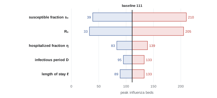
Local elasticities describe small changes around one point. When parameters are uncertain over wide ranges, or interact, a global approach is needed. Two common methods complement each other. In one-at-a-time analysis, each parameter is moved across its plausible range while the others are held at baseline, and the resulting range of the output is recorded. Plotted as horizontal bars sorted by length, the results form a tornado diagram that shows at a glance which parameters matter most. In Monte Carlo uncertainty propagation, all parameters are drawn at random from distributions describing their uncertainty, the model is run for each draw, and the distribution of outputs is summarized by its median and percentiles. This uses the tools of lesson 9 and captures interactions between parameters that one-at-a-time analysis misses.

The goal of sensitivity analysis is not only to put error bars on the output. It also tells us which parameters are worth measuring better, since reducing the uncertainty in an insensitive parameter does little; which assumptions are worth revisiting; and whether a decision is robust, in the sense that the same choice is best across the plausible range of parameters.

Structural uncertainty

Parameters are not the only source of uncertainty. The form of the model itself is an assumption. The logistic, Gompertz and Ricker growth laws give different maximum sustainable yields with the same data; a well-mixed SIR model and an age-structured one give different peaks. Structural uncertainty is assessed by building alternative models on different plausible assumptions and comparing their conclusions. Where they agree, the conclusion is robust; where they differ, the difference is itself a finding that should be reported, together with the data that would distinguish the models. Weather forecasters and climate scientists formalize this approach with ensembles of models, and epidemic forecasting hubs combine the projections of many independent teams.

Capstone: hospital beds for the influenza season

The public health unit asks: how many hospital beds should the city's hospitals plan to make available for influenza patients at the peak of the coming season? We work through the modelling cycle.

Question and assumptions. The output is the number of occupied influenza beds at the peak. We use the SIR model of lesson 7 for the city of 500,000, with three adjustments: a fraction \(s_0\) of the population is susceptible at the start, because of immunity from vaccination and earlier seasons; a fraction \(\eta\) of infections lead to hospital admission; and admitted patients stay an average of \(\ell\) days. At the peak, new infections occur at the rate \(\frac{I_{\max}}{D}\), where \(D = \frac{1}{\gamma}\) is the infectious period, since at the peak \(R_0s = 1\) and the infection rate equals the recovery rate. If the peak is broad compared with the length of stay, occupied beds are about \[B \approx \eta\,\ell\,\frac{I_{\max}}{D}, \qquad I_{\max} = P\Big(s_0 - \frac{1 + \ln(R_0s_0)}{R_0}\Big).\]

Solution and sensitivity. The program below computes the baseline, the elasticities, the one-at-a-time ranges and a Monte Carlo distribution with each parameter drawn uniformly from its range.

import math, random
P = 500_000

def beds(R0=1.5, s0=0.9, eta=0.004, stay=5.0, D=3.0):
    Re = R0 * s0
    if Re <= 1:
        return 0.0
    i_max = s0 - (1 + math.log(Re)) / R0
    return eta * (P * i_max / D) * stay

base = dict(R0=1.5, s0=0.9, eta=0.004, stay=5.0, D=3.0)
b0 = beds(**base)
print(f"baseline peak beds: {b0:.0f}")
ranges = dict(R0=(1.3, 1.7), s0=(0.8, 1.0), eta=(0.003, 0.005), stay=(4.0, 6.0), D=(2.5, 3.5))
print("elasticities:")
for k in base:
    h = 1e-6 * base[k]
    up = dict(base); up[k] += h
    print(f"  {k:5s} {(beds(**up) - b0) / h * base[k] / b0:6.2f}")
print("one-at-a-time ranges:")
for k, (lo, hi) in ranges.items():
    a = dict(base); a[k] = lo; b = dict(base); b[k] = hi
    print(f"  {k:5s} {beds(**a):6.0f} to {beds(**b):6.0f}")
random.seed(12)
samples = sorted(beds(**{k: random.uniform(*ranges[k]) for k in ranges}) for _ in range(20000))
n = len(samples)
print(f"Monte Carlo: median {samples[n // 2]:.0f}, 90% interval {samples[int(0.05 * n)]:.0f} to {samples[int(0.95 * n)]:.0f}")
print(f"P(beds > 300) = {sum(s > 300 for s in samples) / n:.3f}")

baseline peak beds: 111
elasticities:
  R0      6.01
  s0      7.01
  eta     1.00
  stay    1.00
  D      -1.00
one-at-a-time ranges:
  R0        33 to    205
  s0        39 to    210
  eta       83 to    139
  stay      89 to    133
  D        133 to     95
Monte Carlo: median 105, 90% interval 20 to 266
P(beds > 300) = 0.026

Interpretation. The baseline estimate is about 110 beds. But the elasticities show that the answer is dominated by two parameters: \(R_0\), with elasticity about 6, and the susceptible fraction \(s_0\), with elasticity about 7. The hospitalized fraction, length of stay and infectious period have elasticities of exactly 1 or \(-1\), because they enter the formula as factors. Over their plausible ranges, \(R_0\) alone moves the answer from about 30 to 200 beds, and \(s_0\) from about 40 to 210, while the other three move it by less than 30 in either direction.

Recommendation. The Monte Carlo distribution has a median near 105 beds and a 90% interval from about 20 to 270. Planning for the median would leave the hospitals short in roughly half of plausible seasons; planning for about 270 beds covers 95% of the simulated outcomes, and the probability of needing more than 300 is under 3%. The report should therefore recommend a surge plan able to reach 270 beds, with a trigger: as soon as early-season surveillance gives an estimate of the growth rate, \(R_0s_0\) can be estimated from it, as in lesson 7, and the plan updated. Because the output is so sensitive to the effective reproduction number, a better serological survey of immunity before the season would reduce the uncertainty far more than better data on hospital stays.

Limitations. The model is well mixed, while influenza hospitalizations are concentrated among the very young and the old, so an age-structured model could change the estimate. The bed formula assumes a broad peak, and real peaks with strong school effects can be sharper. These limitations do not change the main conclusion, that the plan must allow for a wide range and be updated from early data, but they should be stated so that readers can judge the recommendation.

Writing the modelling report

A modelling report is a scientific argument. Its standard structure, used in this course since lesson 1, is designed to let a reader check every step. Begin with a summary in plain language: the question, the answer, its uncertainty and the recommendation, in a few sentences that a decision maker can read alone. Then state the question precisely and explain why it matters. List the assumptions, each with its justification and an indication of how it might affect the results. Present the model, with a table of variables and parameters giving units, values and sources. Describe the methods of solution and their verification. Present the results with clear figures, each with a caption that states what it shows. Report the sensitivity and uncertainty analysis. Discuss limitations and possible extensions. Finally, include the code or enough detail for someone else to reproduce the results.

Good figures carry much of the argument. Label axes with quantities and units, use the same scales when figures are to be compared, and show uncertainty with bands or intervals rather than single lines. Avoid false precision: reporting 111 beds suggests an accuracy the model does not have, while 'about 110, plausibly between 20 and 270' is honest. Separate what the model shows from what the modeller recommends, since the recommendation also depends on values, such as how much risk of a shortage is acceptable, that are for decision makers to set.

Your capstone: the Larch Lake harvest control rule

The second capstone project draws together the fishery thread of the course and is set as the final assignment. The fisheries office must choose a harvest rule for the next twenty years. Formulate the question, including what counts as success, such as average catch and the probability that the stock falls below 10,000. Use the logistic model fitted in lesson 10, with the uncertainty in \(r\) and \(K\), and the stochastic recruitment of lesson 9. Compare at least three rules: a constant quota, a constant effort, and a threshold rule that reduces effort linearly when the surveyed stock falls below a trigger level. Verify your simulation against the deterministic results of lesson 5. Carry out a sensitivity analysis, including at least one structural alternative such as the Ricker or Gompertz model. Write a report following the structure above, with a one-paragraph summary for the fisheries office and a recommendation that states how robust it is to the uncertainties you have identified.

A model never ends the conversation it was built for; it disciplines it. It makes assumptions explicit, quantifies trade-offs and identifies the data that would most improve a decision. The fishery, the epidemic and the bus route have served as examples, but the methods of this course, from dimensional analysis to Monte Carlo simulation, apply wherever a question can be stated precisely and quantities can be measured. The habits that matter most are the ones the cycle enforces: begin with the question, state every assumption, check units and limiting cases, quantify uncertainty, and go round again when the model fails.