Sensitivity analysis and shadow prices

The data of a real linear program are never exact. Prices fluctuate, capacities are estimates, and managers want to know what would happen if they bought more of a resource or changed a product's price. Sensitivity analysis answers such questions from the optimal solution already computed, without starting over. The key objects are the shadow prices, the optimal dual variables of lesson 6, which measure the marginal value of each constraint, and the ranges over which the current optimal basis stays optimal as one number changes. This lesson proves that shadow prices are derivatives of the optimal value, shows that the optimal value is a piecewise linear function of the right-hand side, derives ranging formulas for right-hand sides and costs, and uses shadow prices to decide whether a new product is worth introducing.

Shadow prices as derivatives

Write the optimal value of the standard form problem, minimize \(c^Tx\) subject to \(Ax = b\), \(x \ge 0\), as a function \(z^*(b)\) of the right-hand side, with the convention that \(z^*(b) = +\infty\) when the problem is infeasible. Suppose \(B\) is an optimal basis for the data \(b\), nondegenerate in the sense that \(x_B = B^{-1}b > 0\).

Theorem. If \(B\) is a nondegenerate optimal basis for \(b\), then for all \(\Delta b\) small enough, \(B\) remains optimal for \(b + \Delta b\), and \(z^*(b + \Delta b) = z^*(b) + y^T\Delta b\), where \(y^T = c_B^TB^{-1}\). In particular \(\partial z^*/\partial b_i = y_i\).

Proof. Changing \(b\) does not change the reduced costs \(c_j - c_B^TB^{-1}A_j\), which do not involve \(b\); they stay nonnegative. The basic solution for \(b + \Delta b\) is \(B^{-1}(b + \Delta b) = x_B + B^{-1}\Delta b\), which stays nonnegative for small \(\Delta b\) because \(x_B > 0\). So \(B\) is still a feasible basis with nonnegative reduced costs, hence optimal, and the optimal value is \(c_B^TB^{-1}(b + \Delta b) = z^*(b) + y^T\Delta b\). \(\square\)

The name shadow price reflects this: \(y_i\) is the price at which an extra unit of resource \(i\) would just break even, an implicit price cast by the optimization rather than set by a market. For the shop of lesson 2, the dual solution \(y = (10, 10, 0)\) says that an extra carpentry hour or an extra finishing hour would each raise the weekly profit by 10 dollars, while extra table demand is worth nothing because demand is not the bottleneck. The shop should pay up to 10 dollars an hour for overtime in either department, and no more. The theorem is local: it holds only while the basis stays optimal, and the next sections find out for how long.

The optimal value as a function of the right side

Theorem. For a maximization in the symmetric form, the optimal value \(z^*(b) = \max\{c^Tx : Ax \le b,\ x \ge 0\}\) is a concave, piecewise linear function of \(b\) on the set of \(b\) where it is finite. For a minimization the optimal value is convex and piecewise linear.

Proof. Where \(z^*(b)\) is finite, strong duality gives \(z^*(b) = \min\{b^Ty : A^Ty \ge c,\ y \ge 0\}\). The dual feasible set does not depend on \(b\); it is a polyhedron containing no line (it lies in \(y \ge 0\)), and by the fundamental theorem the minimum, when finite, is attained at one of its finitely many vertices \(y^{(1)}, \ldots, y^{(K)}\). Hence \(z^*(b) = \min_k b^Ty^{(k)}\), a minimum of finitely many linear functions of \(b\). Such a function is piecewise linear, and it is concave because a minimum of linear (hence concave) functions is concave: for \(b, b'\) and \(0 \le \lambda \le 1\), each \(b^Ty^{(k)}\) is linear, so \(\min_k (\lambda b + (1 - \lambda)b')^Ty^{(k)} \ge \lambda\min_k b^Ty^{(k)} + (1 - \lambda)\min_k b'^Ty^{(k)}\). \(\square\)

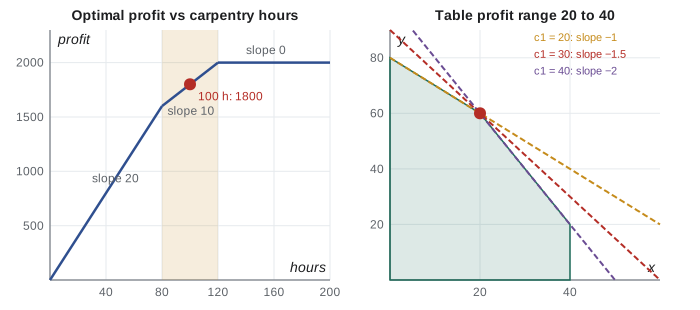
Concavity has an economic meaning, diminishing returns: each extra unit of a resource is worth at most as much as the previous one. As carpentry hours grow, the shop first finds every hour valuable, then less so as finishing becomes the bottleneck, and eventually worthless once demand for tables and the finishing hours are both exhausted.

Ranging the right-hand side

The basis \(B\) remains optimal as \(b_i\) changes to \(b_i + \delta\) exactly as long as the basic solution stays nonnegative: \(x_B + \delta B^{-1}e_i \ge 0\), where \(B^{-1}e_i\) is column \(i\) of \(B^{-1}\). Each component gives a bound on \(\delta\), and together they define an interval, the right-hand-side range, on which the shadow price \(y_i\) is valid. In the final tableau of a problem with slack variables, column \(i\) of \(B^{-1}\) is the column of slack \(s_i\), so the range can be read directly from the tableau.

The same computation for finishing, using the \(s_2\) column \((1, 2, -1)\), gives basic values \((20 + \delta, 60 + 2\delta, 20 - \delta)\), so the range is \(-20 \le \delta \le 20\), that is 60 to 100 finishing hours. For table demand the \(s_3\) column is \((1, 0, 0)\) and the range is \(\delta \ge -20\): the shadow price 0 is valid for any demand of at least 20 tables.

At the end of a range the basis becomes degenerate and the shadow price becomes one-sided. At exactly 120 carpentry hours, the left derivative of the profit is 10 and the right derivative is 0, and every \(y_1\) between 0 and 10 is an optimal dual value. Solvers report one of them, and a careless reading of a reported shadow price at a degenerate optimum can mislead. The honest summary of a shadow price is always a number together with its range.

Ranging the costs

Changing a cost coefficient does not affect feasibility of the current basis, only its optimality, which depends on the reduced costs. If \(c_j\) changes for a nonbasic \(j\), only \(\bar c_j\) changes, by the same amount, so the basis stays optimal while \(\bar c_j\) keeps its sign. If \(c_j\) changes for a basic \(j\), then \(c_B\), hence \(y\), hence every nonbasic reduced cost changes, and each gives a linear inequality in the change.

For the shop with general profits \(c_1\) per table and \(c_2\) per bookcase, the basis with \(x\), \(y\) and \(s_3\) basic has dual prices determined by the tight constraints: \(2y_1 + y_2 = c_1\) and \(y_1 + y_2 = c_2\) give \(y_1 = c_1 - c_2\) and \(y_2 = 2c_2 - c_1\). The basis stays optimal while both are nonnegative:

With \(c_2 = 20\) this is \(20 \le c_1 \le 40\), matching the slope argument of lesson 2, and with \(c_1 = 30\) it is \(15 \le c_2 \le 30\). Inside these ranges the plan \((20, 60)\) does not change at all, though the profit does. When two costs change at once, the ranges for single changes are not enough. A sufficient condition, the hundred per cent rule popularized by Bradley, Hax and Magnanti, says the basis stays optimal if the sum of the fractions of the allowed ranges used by the individual changes is at most one; this follows from convexity of the set of cost vectors for which a basis is optimal.

Pricing out a new activity

Shadow prices also evaluate options that are not yet in the model. Suppose the shop could make desks, each earning 45 dollars and using 3 carpentry hours and 1 finishing hour. At the current shadow prices the resources in a desk are worth \(3 \cdot 10 + 1 \cdot 10 = 40\) dollars. A desk earns more than the value of what it uses, so its reduced profit is \(45 - 40 = 5 > 0\), and introducing desks would increase profit. Had the desk earned less than 40, the current plan would stay optimal with desks added to the model, at no further computation. This test, called pricing out, is exactly the simplex method's choice of entering variable applied to a new column, and it is the basis of column generation, a technique for LPs with too many variables to list, where new columns are generated only when they price out favourably.

When the new activity does price out, a few simplex pivots starting from the current basis find the new optimum. For the desks the new optimum makes 70 bookcases and 10 desks and no tables, earning 1850 dollars, with new shadow prices of 12.50 per carpentry hour and 7.50 per finishing hour. Adding a column changes the shadow prices because the resources now have a new use.

Sensitivity in practice

Sensitivity reports are among the most used outputs of commercial LP solvers, because decision makers rarely trust a single optimal plan from uncertain data but readily use statements such as one more finishing hour is worth 10 dollars, valid from 60 to 100 hours. Three cautions apply. Ranges are for one change at a time. Shadow prices at degenerate optima are one-sided. And sensitivity analysis is local; for large changes in data, or for planning under uncertainty, one re-solves for scenarios, or uses stochastic or robust optimization, which build uncertainty into the model itself.

Sensitivity by re-solving

The program checks the theory by brute force. It re-solves the shop model with each right-hand side increased and decreased by one unit and compares the change in profit with the shadow price; it traces the optimal profit as carpentry hours vary from 0 to 200; it scans for the right-hand side range and the table profit range; and it prices out the desk and then re-solves with desks included.

from fractions import Fraction as Fr

def solve_lp(c, A, b, sense):
    """Minimize c^T x subject to rows A[i] x (sense[i] in '<=', '>=', '=') b[i], x >= 0.
    Exact two-phase simplex with Bland's rule. Returns (status, x, value, y) where y holds
    the dual values (shadow prices) of the rows: y_i = d(optimal value)/d(b_i)."""
    m, n = len(A), len(c)
    rows, rhs, cols = [], [], n
    slack = {}
    for i in range(m):                                  # add slack or surplus columns
        r = [Fr(v) for v in A[i]]
        rows.append(r); rhs.append(Fr(b[i]))
        if sense[i] != '=':
            slack[i] = cols; cols += 1
    for i in range(m):
        rows[i] += [Fr(0)] * (cols - n)
        if i in slack:
            rows[i][slack[i]] = Fr(1 if sense[i] == '<=' else -1)
        if rhs[i] < 0:                                  # make the right side nonnegative
            rows[i] = [-v for v in rows[i]]; rhs[i] = -rhs[i]
    N = cols + m                                        # artificial columns cols .. cols+m-1
    T = [rows[i] + [Fr(int(k == i)) for k in range(m)] + [rhs[i]] for i in range(m)]
    basis = [cols + i for i in range(m)]

    def price(cost):
        z = [Fr(v) for v in cost] + [Fr(0)]
        for i, j in enumerate(basis):
            z = [a - z[j] * q for a, q in zip(z, T[i])]
        return z

    def pivot(r, e):
        p = T[r][e]
        T[r] = [v / p for v in T[r]]
        for i in range(len(T)):
            if i != r and T[i][e] != 0:
                f = T[i][e]; T[i] = [a - f * q for a, q in zip(T[i], T[r])]
        basis[r] = e

    def simplex(allowed):
        while True:
            e = next((j for j in allowed if T[-1][j] < 0), None)   # Bland: smallest index
            if e is None:
                return "optimal"
            rs = [i for i in range(len(T) - 1) if T[i][e] > 0]
            if not rs:
                return "unbounded"
            t = min(T[i][-1] / T[i][e] for i in rs)
            pivot(min((i for i in rs if T[i][-1] / T[i][e] == t), key=lambda i: basis[i]), e)

    T.append(price([0] * cols + [1] * m))               # phase one
    simplex(range(N))
    if T[-1][-1] != 0:
        return "infeasible", None, None, None
    T.pop()
    for i in range(m):                                  # drive zero artificials out if possible
        if basis[i] >= cols:
            e = next((j for j in range(cols) if T[i][j] != 0), None)
            if e is not None:
                pivot(i, e)
    T.append(price(list(c) + [0] * (cols - n) + [0] * m))
    status = simplex(range(cols))                       # phase two on original columns only
    if status != "optimal":
        return status, None, None, None
    x = [Fr(0)] * N
    for i, j in enumerate(basis):
        x[j] = T[i][-1]
    # duals from B^T y = c_B, read off the artificial columns: y = c_B^T B^{-1} (sign-corrected)
    y = [-T[-1][cols + i] for i in range(m)]
    y = [(-v if Fr(b[i]) < 0 else v) for i, v in enumerate(y)]
    return "optimal", x[:n], -T[-1][-1], y

A = [[2, 1], [1, 1], [1, 0]]
names = ["carpentry", "finishing", "demand"]
def profit(b, c=(30, 20), A=A):
    st, x, v, y = solve_lp([-ci for ci in c], A, b, ["<="] * len(b))
    return -v, x, [-t for t in y]

base = [100, 80, 40]
z0, x0, y0 = profit(base)
print(f"base plan {tuple(map(str, x0))}, profit {z0}, shadow prices {tuple(map(str, y0))}")

# 1. shadow prices by re-solving with a perturbed right-hand side
for i in range(3):
    b = list(base); b[i] += 1
    z1, _, _ = profit(b)
    b[i] -= 2
    zm, _, _ = profit(b)
    print(f"{names[i]:9s}: +1 unit -> {z1} (change {z1 - z0:+}), -1 unit -> {zm} (change {zm - z0:+})")

# 2. the optimal profit as a function of carpentry hours: piecewise linear and concave
print("carpentry hours -> optimal profit:")
for h in range(0, 201, 20):
    z, x, y = profit([h, 80, 40])
    print(f"   {h:3d} h: profit {str(z):>5s}, plan ({x[0]}, {x[1]}), shadow price {y[0]}")

# 3. right-hand side range over which the carpentry shadow price stays 10
inside = [h for h in range(60, 141) if profit([h, 80, 40])[2][0] == 10]
print(f"solver reports carpentry price 10 for hours {inside[0]} to {inside[-1]}; "
      f"formula B^-1 b >= 0 gives the closed range [80, 120]")

# 4. cost ranging: table profit range keeping (20, 60) optimal
keep = [p for p in range(10, 51) if 20 * p + 60 * 20 == profit(base, (p, 20))[0]]
print(f"(20, 60) stays optimal for table profits {keep[0]} to {keep[-1]}")

# 5. pricing out a new product: a desk needs 3 h carpentry, 1 h finishing, earns 45
a_new, p_new = (3, 1), 45
worth = sum(ai * yi for ai, yi in zip(a_new, y0))
print(f"desk: resources worth {worth} at current shadow prices, profit {p_new} -> "
      f"{'make some' if p_new > worth else 'do not make'}")
A3 = [[2, 1, 3], [1, 1, 1], [1, 0, 0]]
z3, x3, y3 = profit(base, (30, 20, 45), A3)
print(f"with desks: plan (tables, bookcases, desks) = {tuple(map(str, x3))}, profit {z3}, "
      f"new shadow prices {tuple(map(str, y3))}")

base plan ('20', '60'), profit 1800, shadow prices ('10', '10', '0')
carpentry: +1 unit -> 1810 (change +10), -1 unit -> 1790 (change -10)
finishing: +1 unit -> 1810 (change +10), -1 unit -> 1790 (change -10)
demand   : +1 unit -> 1800 (change +0), -1 unit -> 1800 (change +0)
carpentry hours -> optimal profit:
     0 h: profit     0, plan (0, 0), shadow price 20
    20 h: profit   400, plan (0, 20), shadow price 20
    40 h: profit   800, plan (0, 40), shadow price 20
    60 h: profit  1200, plan (0, 60), shadow price 20
    80 h: profit  1600, plan (0, 80), shadow price 20
   100 h: profit  1800, plan (20, 60), shadow price 10
   120 h: profit  2000, plan (40, 40), shadow price 10
   140 h: profit  2000, plan (40, 40), shadow price 0
   160 h: profit  2000, plan (40, 40), shadow price 0
   180 h: profit  2000, plan (40, 40), shadow price 0
   200 h: profit  2000, plan (40, 40), shadow price 0
solver reports carpentry price 10 for hours 81 to 120; formula B^-1 b >= 0 gives the closed range [80, 120]
(20, 60) stays optimal for table profits 20 to 40
desk: resources worth 40 at current shadow prices, profit 45 -> make some
with desks: plan (tables, bookcases, desks) = ('0', '70', '10'), profit 1850, new shadow prices ('25/2', '15/2', '0')

Each finite difference equals the shadow price exactly, as the theorem promises for a nondegenerate basis. The profit table traces a concave broken line with slopes 20, 10 and 0, and the solver's reported carpentry price at the breakpoints 80 and 120 hours illustrates the one-sided behaviour at degenerate vertices: at 80 hours it reports the slope 20 to the left, and at 120 hours the slope 10 to the left. The table profit range 20 to 40 agrees with \(c_2 \le c_1 \le 2c_2\). Finally, the desk prices out at a reduced profit of 5 and the re-solved plan earns 1850, with new shadow prices \(\frac{25}{2}\) and \(\frac{15}{2}\).