
MATH-372 · Lesson 6 of 12 · 24 min
Duality and complementary slackness
Every linear program has a twin, its dual, built from the same data read sideways. The dual of a maximization is a minimization, its variables correspond to the primal constraints, and its constraints correspond to the primal variables. The two problems are bound together by the duality theorem: when either has an optimal solution, so does the other, and their optimal values are equal. This is the central result of linear programming. It provides short certificates of optimality, turns the final simplex tableau into economic prices, gives a criterion for checking a claimed optimum by hand, and leads to the theorems of the alternative, such as Farkas's lemma, that pervade optimization. This lesson constructs the dual, proves weak and strong duality, and develops complementary slackness.
Bounding the optimum
Return to the shop of lesson 2: maximize \(30x + 20y\) subject to \(2x + y \le 100\), \(x + y \le 80\), \(x \le 40\), \(x, y \ge 0\). Without solving, can we prove that the profit can never exceed some number? Multiply the carpentry constraint by 15: \(30x + 15y \le 1500\). Since \(y \ge 0\), \(30x + 20y \le 30x + 15y + 5y\), which is not obviously bounded. Try instead adding 10 times the carpentry constraint and 10 times the finishing constraint: \(30x + 20y \le 1000 + 800 = 1800\). Because the left side is exactly the profit, every feasible plan earns at most 1800, and the plan \((20, 60)\) earning 1800 is therefore optimal. The multipliers \((10, 10, 0)\) are a certificate.
In general, multiply the constraints by \(y_1, y_2, y_3 \ge 0\) (nonnegative, so the inequalities keep their direction) and add: \((2y_1 + y_2 + y_3)x + (y_1 + y_2)y \le 100y_1 + 80y_2 + 40y_3\). If the coefficient of \(x\) is at least 30 and that of \(y\) at least 20, then, since \(x, y \ge 0\), the profit is at most the right side. The best bound of this kind solves another LP:
This is the dual of the shop problem. It has a pleasing economic reading. An investor offers to rent all the shop's resources, paying \(y_1\) per carpentry hour, \(y_2\) per finishing hour and \(y_3\) per unit of table demand. The shop will accept only if the rent for the resources in a table is at least the 30 dollars a table would earn, and likewise for bookcases; the investor wants to pay as little as possible. The investor's minimal total rent equals the shop's maximal profit, 1800, at prices \(y = (10, 10, 0)\).
The dual in general
For the symmetric form, the primal (P) and dual (D) are
For the standard form used by the simplex method, the pair is
The equality constraints give free dual variables because multipliers of equations may have either sign. Both pairs follow from one dictionary, which also shows that the dual of the dual is the primal. For a minimization primal:
| Minimization primal | Maximization dual |
|---|---|
| Constraint i: row i of Ax ≥ b_i | Variable y_i ≥ 0 |
| Constraint i: row i of Ax ≤ b_i | Variable y_i ≤ 0 |
| Constraint i: row i of Ax = b_i | Variable y_i free |
| Variable x_j ≥ 0 | Constraint j: column j of A, dotted with y, ≤ c_j |
| Variable x_j ≤ 0 | Constraint j: column j of A, dotted with y, ≥ c_j |
| Variable x_j free | Constraint j: column j of A, dotted with y, = c_j |
| Objective c^T x | Objective b^T y |
Worked problem
Dual of the feed blend
Write the dual of the feed blend of lesson 2: minimize \(0.30x_1 + 0.90x_2\) subject to \(x_1 + x_2 \ge 800\), \(-0.21x_1 + 0.30x_2 \ge 0\), \(0.03x_1 - 0.01x_2 \ge 0\), \(x \ge 0\).
Show solution
- Three \(\ge\) constraints in a minimization give dual variables \(y_1, y_2, y_3 \ge 0\).
- Two nonnegative primal variables give two \(\le\) dual constraints, one per column: \(y_1 - 0.21y_2 + 0.03y_3 \le 0.30\) and \(y_1 + 0.30y_2 - 0.01y_3 \le 0.90\).
- The dual objective is \(800y_1\), to be maximized.
- At the primal optimum the protein and quantity rows are tight and the fibre row has slack, which suggests \(y_3 = 0\) with both dual constraints tight: \(y_1 - 0.21y_2 = 0.30\), \(y_1 + 0.30y_2 = 0.90\), giving \(y_2 = 0.60/0.51 \approx 1.176\), \(y_1 \approx 0.547\).
Answer: The dual optimum is \(800y_1 \approx 437.65\), matching the primal cost. Here \(y_1 \approx 0.547\) dollars per kg is the marginal cost of feed: producing 801 kg would cost about 55 cents more.
Weak duality
Theorem (weak duality). If \(x\) is feasible for (P) and \(y\) is feasible for (D) in the symmetric pair, then \(c^Tx \le b^Ty\).
Proof. Using \(x \ge 0\) with \(A^Ty \ge c\), and \(y \ge 0\) with \(Ax \le b\): \(c^Tx \le (A^Ty)^Tx = y^TAx \le y^Tb\). \(\square\)
The proof is just the bounding argument of the shop example in matrix form. Three corollaries follow at once. If (P) is unbounded, (D) is infeasible, since a feasible \(y\) would bound \(c^Tx\). If (D) is unbounded, (P) is infeasible. And if feasible \(x\) and \(y\) satisfy \(c^Tx = b^Ty\), both are optimal, since no primal value can exceed \(b^Ty\) and no dual value can fall below \(c^Tx\). The last corollary is the certificate idea: a dual solution with matching value proves primal optimality in one inequality check.
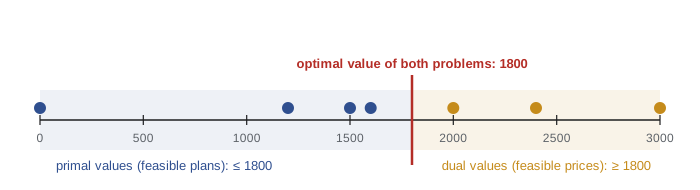
Strong duality
Theorem (strong duality). If (P) has an optimal solution, so does (D), and the optimal values are equal. Here (P) is the standard form, minimize \(c^Tx\) subject to \(Ax = b\), \(x \ge 0\).
Proof. By lesson 5, the simplex method with Bland's rule, preceded by phase one, terminates; since (P) has an optimum, it terminates with an optimal basis \(B\) whose reduced costs are nonnegative: \(c_j - c_B^TB^{-1}A_j \ge 0\) for every \(j\). (If phase one left redundant rows, delete them; they do not affect either problem, and the dual variables for deleted rows can be set to zero.) Define \(y\) by \(y^T = c_B^TB^{-1}\). The reduced cost conditions say exactly \(A_j^Ty \le c_j\) for all \(j\), that is \(A^Ty \le c\), so \(y\) is dual feasible. Its value is \(b^Ty = c_B^TB^{-1}b = c_B^Tx_B = c^Tx\), the primal optimal value. By the weak duality corollary, \(y\) is dual optimal. \(\square\)
The proof shows more than equality of values: the optimal dual solution can be read from the optimal basis as \(y^T = c_B^TB^{-1}\), the simplex multipliers. In the shop tableau of lesson 4 the reduced profits of the slack columns were \(-10, -10, 0\); their negatives are the dual optimum \((10, 10, 0)\). Applying the theorem to the dual (after rewriting it in standard form), and using that the dual of the dual is the primal, gives the symmetric statement: if (D) has an optimum, so does (P). Together with weak duality this leaves exactly four possibilities for a primal–dual pair: both have optima with equal values; (P) is unbounded and (D) infeasible; (D) is unbounded and (P) infeasible; or both are infeasible. The last really happens, for instance with \(\max x_1\) subject to \(x_1 - x_2 \le -1\), \(-x_1 + x_2 \le -1\), \(x \ge 0\), whose constraints add to \(0 \le -2\), and whose dual is infeasible for a similar reason.
The duality theorem has a famous origin story. In October 1947 Dantzig visited John von Neumann in Princeton to describe linear programming. Von Neumann, who with Oskar Morgenstern had just published the theory of games built on his 1928 minimax theorem, immediately conjectured the duality theorem, recognizing that LP and two-person zero-sum games were equivalent. The first published rigorous proof was by David Gale, Harold Kuhn and Albert Tucker in 1951.
Farkas's lemma
Duality yields theorems of the alternative, which say that exactly one of two systems has a solution. The most important is due to Gyula Farkas, who published it in 1902.
Theorem (Farkas's lemma). For a matrix \(A\) and vector \(b\), exactly one of the following holds: (i) there is \(x \ge 0\) with \(Ax = b\); (ii) there is \(y\) with \(A^Ty \ge 0\) and \(b^Ty < 0\).
Proof. Both cannot hold: if \(Ax = b\), \(x \ge 0\) and \(A^Ty \ge 0\), then \(b^Ty = x^TA^Ty \ge 0\). Now suppose (i) fails. Consider (P): minimize \(0^Tx\) subject to \(Ax = b\), \(x \ge 0\), which is infeasible, and its dual (D): maximize \(b^Ty\) subject to \(A^Ty \le 0\). The dual is feasible, with \(y = 0\). If (D) had an optimum, strong duality applied to (D), rewritten in standard form, would give its dual (P) an optimum, which is impossible. So (D) is unbounded: some feasible \(y\) has \(b^Ty > 0\). Then \(-y\) satisfies \(A^T(-y) \ge 0\) and \(b^T(-y) < 0\), which is (ii). \(\square\)
Geometrically, (i) says \(b\) lies in the cone generated by the columns of \(A\); (ii) gives a hyperplane through the origin, with normal \(y\), that has all the columns on one side and \(b\) strictly on the other. The vector \(y\) is a certificate of infeasibility, the counterpart for infeasible problems of the dual certificate of optimality. Solvers return one when they declare a problem infeasible. Lesson 11 uses Farkas's lemma to derive the Karush–Kuhn–Tucker conditions.
Complementary slackness
Theorem (complementary slackness). Let \(x\) be feasible for the symmetric (P) and \(y\) feasible for (D). Then both are optimal if and only if
Proof. The weak duality chain \(c^Tx \le y^TAx \le y^Tb\) can be rewritten as \(b^Ty - c^Tx = y^T(b - Ax) + x^T(A^Ty - c)\). Both terms on the right are sums of products of nonnegative numbers, so the gap is zero exactly when every product is zero. By strong duality and its corollary, the gap is zero exactly when both are optimal. \(\square\)
In words: if a resource has a positive price, it is fully used; if a resource is not fully used, its price is zero; if a product is made, its resources are worth exactly its profit; and if the resources in a product are worth more than its profit, it is not made. For the shop, table demand is not exhausted (slack 20), so its price \(y_3\) is zero, while carpentry and finishing, fully used, have positive prices.
Complementary slackness turns a guess into a proof. Given a claimed primal optimum, the conditions determine which dual constraints must be tight and which dual variables must vanish, often leaving a square linear system for \(y\). If its solution is dual feasible, the claim is proved; if not, the claim is false. This is how the feed blend dual was found above, and how the program below verifies the shop plan.
Primal and dual in code
The program contains a compact exact two-phase simplex solver (the methods of lessons 4 and 5) that also returns the simplex multipliers. It solves the shop problem and its dual separately, compares the dual solution with the shadow prices read from the primal, checks strong duality and every complementary slackness product, illustrates weak duality with feasible points of each problem, and finally verifies the plan \((20, 60)\) by complementary slackness alone.
from fractions import Fraction as Fr

def solve_lp(c, A, b, sense):
    """Minimize c^T x subject to rows A[i] x (sense[i] in '<=', '>=', '=') b[i], x >= 0.
    Exact two-phase simplex with Bland's rule. Returns (status, x, value, y) where y holds
    the dual values (shadow prices) of the rows: y_i = d(optimal value)/d(b_i)."""
    m, n = len(A), len(c)
    rows, rhs, cols = [], [], n
    slack = {}
    for i in range(m):                                  # add slack or surplus columns
        r = [Fr(v) for v in A[i]]
        rows.append(r); rhs.append(Fr(b[i]))
        if sense[i] != '=':
            slack[i] = cols; cols += 1
    for i in range(m):
        rows[i] += [Fr(0)] * (cols - n)
        if i in slack:
            rows[i][slack[i]] = Fr(1 if sense[i] == '<=' else -1)
        if rhs[i] < 0:                                  # make the right side nonnegative
            rows[i] = [-v for v in rows[i]]; rhs[i] = -rhs[i]
    N = cols + m                                        # artificial columns cols .. cols+m-1
    T = [rows[i] + [Fr(int(k == i)) for k in range(m)] + [rhs[i]] for i in range(m)]
    basis = [cols + i for i in range(m)]

    def price(cost):
        z = [Fr(v) for v in cost] + [Fr(0)]
        for i, j in enumerate(basis):
            z = [a - z[j] * q for a, q in zip(z, T[i])]
        return z

    def pivot(r, e):
        p = T[r][e]
        T[r] = [v / p for v in T[r]]
        for i in range(len(T)):
            if i != r and T[i][e] != 0:
                f = T[i][e]; T[i] = [a - f * q for a, q in zip(T[i], T[r])]
        basis[r] = e

    def simplex(allowed):
        while True:
            e = next((j for j in allowed if T[-1][j] < 0), None)   # Bland: smallest index
            if e is None:
                return "optimal"
            rs = [i for i in range(len(T) - 1) if T[i][e] > 0]
            if not rs:
                return "unbounded"
            t = min(T[i][-1] / T[i][e] for i in rs)
            pivot(min((i for i in rs if T[i][-1] / T[i][e] == t), key=lambda i: basis[i]), e)

    T.append(price([0] * cols + [1] * m))               # phase one
    simplex(range(N))
    if T[-1][-1] != 0:
        return "infeasible", None, None, None
    T.pop()
    for i in range(m):                                  # drive zero artificials out if possible
        if basis[i] >= cols:
            e = next((j for j in range(cols) if T[i][j] != 0), None)
            if e is not None:
                pivot(i, e)
    T.append(price(list(c) + [0] * (cols - n) + [0] * m))
    status = simplex(range(cols))                       # phase two on original columns only
    if status != "optimal":
        return status, None, None, None
    x = [Fr(0)] * N
    for i, j in enumerate(basis):
        x[j] = T[i][-1]
    # duals from B^T y = c_B, read off the artificial columns: y = c_B^T B^{-1} (sign-corrected)
    y = [-T[-1][cols + i] for i in range(m)]
    y = [(-v if Fr(b[i]) < 0 else v) for i, v in enumerate(y)]
    return "optimal", x[:n], -T[-1][-1], y

def show(v):
    return "(" + ", ".join(str(t) for t in v) + ")"

# primal: maximize 30x + 20y s.t. A x <= b, x >= 0  (solved as: minimize -30x - 20y)
A = [[2, 1], [1, 1], [1, 0]]
b = [100, 80, 40]
c = [30, 20]
st, x, val, y_shadow = solve_lp([-v for v in c], A, b, ["<="] * 3)
print(f"primal: {st}, x = {show(x)}, profit {-val}")

# dual: minimize b^T y s.t. A^T y >= c, y >= 0 (one dual variable per primal row)
At = [[A[i][j] for i in range(len(A))] for j in range(len(c))]
st, y, dval, _ = solve_lp(b, At, c, [">="] * len(c))
print(f"dual:   {st}, y = {show(y)}, value {dval}")
print("shadow prices read from the primal:", show(-v for v in y_shadow))
print("strong duality c^T x = b^T y:", sum(ci * xi for ci, xi in zip(c, x)) == sum(bi * yi for bi, yi in zip(b, y)))

# complementary slackness: y_i * (b - A x)_i = 0 and x_j * (A^T y - c)_j = 0
slack_p = [b[i] - sum(A[i][j] * x[j] for j in range(2)) for i in range(3)]
slack_d = [sum(At[j][i] * y[i] for i in range(3)) - c[j] for j in range(2)]
print("primal slacks", show(slack_p), " products y_i * slack_i", show(yi * s for yi, s in zip(y, slack_p)))
print("dual surpluses", show(slack_d), " products x_j * surplus_j", show(xj * s for xj, s in zip(x, slack_d)))

# weak duality: any feasible plan earns at most any feasible dual price system charges
plans = [(0, 0), (40, 0), (30, 30), (20, 60)]
prices = [(30, 0, 0), (20, 0, 10), (10, 10, 0), (0, 30, 0)]
for p in plans:
    assert all(sum(A[i][j] * p[j] for j in range(2)) <= b[i] for i in range(3))
for q in prices:
    assert all(sum(At[j][i] * q[i] for i in range(3)) >= c[j] for j in range(2))
print("feasible profits:", [30 * p[0] + 20 * p[1] for p in plans])
print("feasible dual values:", [sum(bi * qi for bi, qi in zip(b, q)) for q in prices])

# using complementary slackness to verify a claimed optimum without solving the LP
claim = (20, 60)
tight = [i for i in range(3) if sum(A[i][j] * claim[j] for j in range(2)) == b[i]]
# x > 0 in both coordinates, so both dual constraints must be tight; y_i = 0 for slack rows
(a11, a12), (a21, a22) = [[At[j][i] for i in tight] for j in range(2)]
det = Fr(a11 * a22 - a12 * a21)
yt = ((c[0] * a22 - a12 * c[1]) / det, (a11 * c[1] - c[0] * a21) / det)
ycl = [Fr(0)] * 3
for i, v in zip(tight, yt):
    ycl[i] = v
print("claimed plan", claim, "tight rows", [i + 1 for i in tight], "-> dual candidate", show(ycl),
"nonnegative:", all(v >= 0 for v in ycl), "so the plan is optimal")primal: optimal, x = (20, 60), profit 1800 dual: optimal, y = (10, 10, 0), value 1800 shadow prices read from the primal: (10, 10, 0) strong duality c^T x = b^T y: True primal slacks (0, 0, 20) products y_i * slack_i (0, 0, 0) dual surpluses (0, 0) products x_j * surplus_j (0, 0) feasible profits: [0, 1200, 1500, 1800] feasible dual values: [3000, 2400, 1800, 2400] claimed plan (20, 60) tight rows [1, 2] -> dual candidate (10, 10, 0) nonnegative: True so the plan is optimal
The dual solved on its own gives \(y = (10, 10, 0)\), identical to the multipliers recovered from the primal's final basis. All five complementary slackness products vanish: demand has slack 20 and price 0, and both products are made with zero dual surplus. The feasible profits listed are all at most 1800 and the feasible dual values all at least 1800, as weak duality requires, and the last line shows how three lines of arithmetic certify the plan without running the simplex method at all.
Common mistakes
MistakeGiving the dual of a \(\le\)-constrained maximization negative variables.
InsteadFor max with \(\le\) rows the dual variables are nonnegative; check signs with the bounding argument or the table.
MistakeForgetting that equality constraints produce free dual variables.
InsteadMultipliers of equations may have either sign.
MistakeConcluding from weak duality that the values are always equal.
InsteadWeak duality gives an inequality; equality needs strong duality and requires an optimum to exist.
MistakeBelieving that if the primal is infeasible the dual must be unbounded.
InsteadBoth can be infeasible.
MistakeReading complementary slackness as "a slack constraint has a positive price".
InsteadIt is the reverse: a slack constraint has a zero price, and a positive price forces the constraint to be tight.
Summary and key terms
- The dual of \(\max c^Tx\), \(Ax \le b\), \(x \ge 0\) is \(\min b^Ty\), \(A^Ty \ge c\), \(y \ge 0\); the dual of the dual is the primal.
- Weak duality: every primal value is at most every dual value, so matching values certify optimality.
- Strong duality: if either problem has an optimum, both do, with equal values; \(y^T = c_B^TB^{-1}\) from the optimal basis is dual optimal.
- A primal–dual pair has equal optima, one unbounded and the other infeasible, or both infeasible.
- Farkas: exactly one of \(Ax = b, x \ge 0\) and \(A^Ty \ge 0, b^Ty < 0\) is solvable.
- Complementary slackness: optimal \(x, y\) make every product of a variable and the slack of its partner constraint zero.
- dual problem
- The LP whose variables are multipliers of the primal constraints and whose value bounds the primal value.
- weak duality
- The inequality between primal and dual objective values for feasible points.
- strong duality
- Equality of the primal and dual optimal values when an optimum exists.
- simplex multipliers
- The vector c_B transpose times B inverse, which is dual optimal at an optimal basis.
- Farkas lemma
- A theorem of the alternative characterizing when Ax = b has a nonnegative solution.
- complementary slackness
- The condition that each dual variable times the slack of its primal constraint is zero, and vice versa.
Practice problems
Work each problem on paper first, then reveal the answer to check.
Write the dual of: minimize \(3x_1 + 2x_2\) subject to \(x_1 + x_2 \ge 4\), \(x_1 - x_2 \le 2\), \(x \ge 0\).
Show answer
Maximize \(4y_1 + 2y_2\) subject to \(y_1 + y_2 \le 3\), \(y_1 - y_2 \le 2\), \(y_1 \ge 0\), \(y_2 \le 0\).
Solve the problem in the previous exercise and verify with its dual.
Show answer
The optimum is \(x = (0, 4)\) with value 8. The dual \(y = (2, 0)\) is feasible (\(2 \le 3\), \(2 \le 2\)) with value 8, so both are optimal.
Use complementary slackness to test whether \(x = (40, 20)\) is optimal for the shop.
Show answer
Tight rows are carpentry and demand, so \(y_2 = 0\). Both \(x, y > 0\), so \(2y_1 + y_3 = 30\) and \(y_1 = 20\), giving \(y_3 = -10 < 0\). Not dual feasible, so \((40, 20)\) is not optimal.
Prove that the dual of the dual of the symmetric pair is the primal.
Show answer
Write (D) as \(\max (-b)^Ty\) s.t. \((-A^T)y \le -c\), \(y \ge 0\). Its symmetric dual is \(\min (-c)^Tx\) s.t. \((-A)x \ge -b\), \(x \ge 0\), which is \(\max c^Tx\) s.t. \(Ax \le b\), \(x \ge 0\).
Find a Farkas certificate showing \(x_1 + x_2 = -1\), \(x \ge 0\) has no solution.
Show answer
\(y = 1\): \(A^Ty = (1, 1) \ge 0\) and \(b^Ty = -1 < 0\).
In the feed dual, explain why \(y_3 = 0\).
Show answer
The fibre constraint has slack at the optimum (\(10.8 > 0\)), so complementary slackness forces its multiplier to vanish.
Lesson quiz · 5 questions
Score 60% or more to complete this lesson.
Create a free account to save your progress, take quizzes and earn a certificate.