
MATH-372 · Lesson 4 of 12 · 27 min
The simplex method
The fundamental theorem of lesson 3 reduced linear programming to a finite search over basic feasible solutions, but the number of them can be astronomically large. In 1947 George Dantzig, then a mathematical adviser to the United States Air Force, proposed a far better strategy: start at a vertex, and repeatedly move along an edge to an adjacent vertex with a better objective value, until no edge improves. Because each step is guided by a simple algebraic test, and because a local optimum of a linear program over a convex polyhedron is global, the walk ends at an optimal vertex. This lesson derives the method in matrix form, proves that its stopping test certifies optimality, works through the tableau mechanics by hand on the shop model, implements it in exact arithmetic, and discusses how many steps it takes.
Moving along an edge
Work with the standard form: minimize \(c^Tx\) subject to \(Ax = b\), \(x \ge 0\), with \(A\) of size \(m \times n\) and rank \(m\). Fix a basis \(B\) (a set of \(m\) column indices with invertible basis matrix, also written \(B\)) whose basic solution is feasible, and let \(N\) be the remaining nonbasic indices. Every solution of \(Ax = b\) can be written in terms of its nonbasic part, because \(Bx_B + Nx_N = b\) gives
Substituting into the objective expresses the cost through the nonbasic variables alone:
The coefficient of \(x_j\) in the bracket, \(\bar c_j = c_j - c_B^TB^{-1}A_j\), is the reduced cost of variable \(j\). It measures the rate at which the objective changes if \(x_j\) is raised from zero while the other nonbasic variables stay at zero and the basic variables adjust to keep \(Ax = b\). For basic variables the same formula gives \(\bar c_j = 0\). At the current vertex \(x_N = 0\), so the objective value is \(c_B^TB^{-1}b\).
Theorem (optimality test). If every reduced cost is nonnegative, \(\bar c \ge 0\), the current basic feasible solution is optimal.
Proof. Let \(y\) be any feasible point. By the identity above, \(c^Ty = c_B^TB^{-1}b + \bar c_N^Ty_N = c^Tx + \bar c_N^Ty_N\). Since \(\bar c_N \ge 0\) and \(y_N \ge 0\), the last term is nonnegative, so \(c^Ty \ge c^Tx\). \(\square\)
The converse holds for nondegenerate vertices: if some \(\bar c_j < 0\) and the vertex is nondegenerate, raising \(x_j\) a little lowers the cost, so the vertex is not optimal. At a degenerate vertex, a negative reduced cost may fail to give improvement, which is the subject of lesson 5.
Suppose then that \(\bar c_j < 0\) for some nonbasic \(j\). Raise \(x_j\) to \(\theta \ge 0\). The basic variables change to \(x_B - \theta u\) where \(u = B^{-1}A_j\), and the cost changes by \(\theta\bar c_j\). Feasibility requires \(x_B - \theta u \ge 0\). If \(u \le 0\), every \(\theta \ge 0\) is allowed and the cost falls without bound: the LP is unbounded, and we have found a ray of the feasible set along which the cost tends to \(-\infty\). Otherwise the largest allowed step is given by the minimum ratio test
At \(\theta = \theta^*\) the basic variable \(x_{B(\ell)}\) reaches zero. It leaves the basis and \(x_j\) enters: the new basis is \(B\) with \(B(\ell)\) replaced by \(j\).
Theorem (pivot). The new columns are linearly independent and the new point \(x + \theta^*d\) is the basic feasible solution of the new basis, where \(d_j = 1\), \(d_B = -u\) and \(d\) is zero elsewhere. Its cost is \(c^Tx + \theta^*\bar c_j \le c^Tx\), with strict decrease when \(\theta^* > 0\).
Proof. If the new columns were dependent, \(A_j\) would be a combination of the columns \(A_{B(i)}\), \(i \ne \ell\). But \(A_j = Bu = \sum_i u_iA_{B(i)}\) with \(u_\ell > 0\), and the expansion in the basis \(B\) is unique, so \(A_j\) genuinely involves \(A_{B(\ell)}\): a contradiction. The new point satisfies \(Ax = b\) since \(Ad = A_j - Bu = 0\), is nonnegative by the choice of \(\theta^*\), and is zero outside the new basis, so it is the new basis's basic feasible solution. The cost change was computed above. \(\square\)
Geometrically, \(d\) points along an edge of the polyhedron leaving the current vertex, and the ratio test stops at the next vertex on that edge. If \(\theta^* = 0\), which happens only when some basic variable in the ratio test is already zero, the basis changes but the point does not: a degenerate pivot.
The algorithm
Collecting the pieces, one iteration of the (revised) simplex method from a basic feasible solution is: compute the reduced costs; if all are nonnegative, stop with an optimal solution; otherwise choose an entering \(j\) with \(\bar c_j < 0\); compute \(u = B^{-1}A_j\); if \(u \le 0\), stop with an unbounded ray; otherwise do the ratio test, choose a leaving index \(\ell\) achieving the minimum, and update the basis.
Theorem (finite termination). If every basic feasible solution is nondegenerate, the simplex method stops after finitely many iterations, either with an optimal basis or with a proof of unboundedness.
Proof. Nondegeneracy means every \(x_{B(i)} > 0\), so every ratio test gives \(\theta^* > 0\) and the cost decreases strictly at each pivot. Hence no basis can be visited twice, since a basis determines its cost. There are finitely many bases, at most \(\binom{n}{m}\), so the method stops. \(\square\)
The choice of entering variable is called the pivoting rule. Dantzig's original rule picks the most negative reduced cost, the steepest rate of improvement per unit of the entering variable. Bland's rule, proposed by Robert Bland in 1977, picks the smallest index with negative reduced cost and breaks ties in the ratio test by the smallest basic index; lesson 5 shows it never cycles even under degeneracy. Production solvers use steepest-edge rules, which normalize the rate by the length of the edge direction, and are usually much faster in practice.
The tableau
For hand computation it is convenient to keep everything in one array, the simplex tableau. For the textbook form, maximize \(c^Tx\) subject to \(Ax \le b\), \(x \ge 0\) with \(b \ge 0\), the slack variables give an obvious starting basis at the origin. Each row stores a constraint in the form currently solved for its basic variable, and the last row stores the reduced profits, the negatives of the reduced costs of the equivalent minimization, together with the negative of the current objective value. Optimality now means no positive entry in the last row. Here is the starting tableau for the shop model of lesson 2.
| Basis | x | y | s1 | s2 | s3 | Right side |
|---|---|---|---|---|---|---|
| s1 | 2 | 1 | 1 | 0 | 0 | 100 |
| s2 | 1 | 1 | 0 | 1 | 0 | 80 |
| s3 | 1 | 0 | 0 | 0 | 1 | 40 |
| Reduced profit | 30 | 20 | 0 | 0 | 0 | 0 |
Worked problem
The first pivot by hand
Carry out one pivot of the shop tableau using Bland's rule.
Show solution
- Entering variable: the positive reduced profits are 30 for \(x\) and 20 for \(y\); Bland's rule takes the smallest index, \(x\) (Dantzig's rule also picks \(x\), the largest).
- Ratio test on the \(x\) column: \(100/2 = 50\), \(80/1 = 80\), \(40/1 = 40\). The minimum is 40 in the \(s_3\) row, so \(s_3\) leaves. The pivot element is the 1 in row \(s_3\), column \(x\).
- Divide the pivot row by the pivot element (here 1). Then subtract multiples of it from the other rows to clear the \(x\) column: row \(s_1\) minus 2 times the pivot row gives \((0, 1, 1, 0, -2 \mid 20)\); row \(s_2\) minus the pivot row gives \((0, 1, 0, 1, -1 \mid 40)\); the profit row minus 30 times the pivot row gives \((0, 20, 0, 0, -30 \mid -1200)\).
- The new basis is \(\{s_1, s_2, x\}\) with basic solution \(s_1 = 20\), \(s_2 = 40\), \(x = 40\) and \(y = s_3 = 0\): the vertex \((40, 0)\) with profit 1200.
Answer: One pivot moved from \((0, 0)\) to the adjacent vertex \((40, 0)\) and raised the profit from 0 to 1200. The positive entry 20 under \(y\) shows the method is not finished.
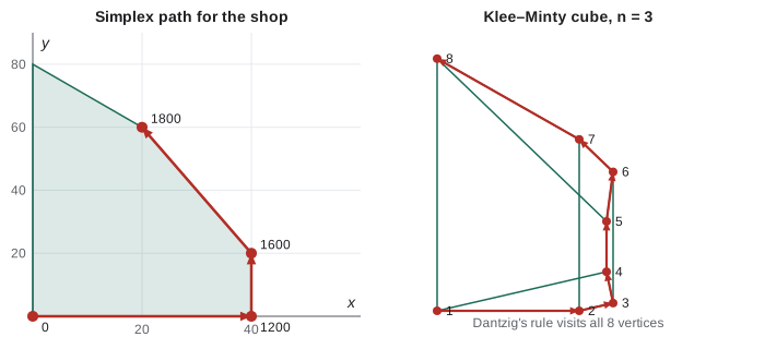
Two more pivots finish the job. Next \(y\) enters, and the ratio test (20 in row \(s_1\), 40 in row \(s_2\)) sends \(s_1\) out, reaching \((40, 20)\) with profit 1600. Then the profit row has a positive entry 10 under \(s_3\): releasing some of the demand constraint, that is making fewer tables, and using the freed carpentry for bookcases pays off. The ratio test in the \(s_3\) column, which has a negative entry in the \(y\) row, compares only \(20/1\) in row \(s_2\) and \(40/1\) in row \(x\), so \(s_2\) leaves. The final tableau is below.
| Basis | x | y | s1 | s2 | s3 | Right side |
|---|---|---|---|---|---|---|
| s3 | 0 | 0 | −1 | 1 | 1 | 20 |
| y | 0 | 1 | −1 | 2 | 0 | 60 |
| x | 1 | 0 | 1 | −1 | 0 | 20 |
| Reduced profit | 0 | 0 | −10 | −10 | 0 | −1800 |
Every entry of the last row is now nonpositive, so by the optimality test the vertex \((20, 60)\) is optimal, confirming the picture of lesson 2. The final row says more. The reduced profit \(-10\) under \(s_1\) means that forcing one hour of carpentry to sit idle would cost 10 dollars of profit, so an extra hour of carpentry is worth 10 dollars; likewise for finishing. These numbers are the shadow prices of lessons 6 and 7, and they come free with the final tableau. The rows also show how the optimum responds to changes: the \(x\) row reads \(x = 20 - s_1 + s_2\) and the \(y\) row reads \(y = 60 + s_1 - 2s_2\), so one extra hour of carpentry (\(s_1 = -1\)) means one more table and one fewer bookcase, while one extra hour of finishing (\(s_2 = -1\)) means one fewer table and two more bookcases.
How many pivots?
Each pivot costs about \(m n\) arithmetic operations in tableau form, so the running time depends on how many pivots are needed. In practice, experience since the 1950s has been that the simplex method typically takes a small multiple of \(m\) pivots, which made it one of the most used algorithms of the twentieth century. In theory the picture is different. In 1972 Victor Klee and George Minty constructed a slightly squashed \(n\)-dimensional cube on which Dantzig's rule visits all \(2^n\) vertices before reaching the optimum. One version is
whose optimum is \(x = (0, \ldots, 0, 5^n)\) with value \(5^n\). Similar exponential examples were later found for every specific pivoting rule studied in detail, including Bland's. Whether some pivoting rule always takes a polynomial number of steps remains a famous open problem, closely tied to the question of the largest possible diameter of a polytope's graph; the Hirsch conjecture that this diameter is at most \(m - n\) was disproved by Francisco Santos in 2010, but no polynomial bound is known.
Two lines of work explain the practical success. Probabilistic analyses by Karl Heinz Borgwardt and Stephen Smale in the early 1980s showed polynomial average behaviour on random problems, and in 2001 Daniel Spielman and Shang-Hua Teng introduced smoothed analysis, proving that a small random perturbation of any LP makes the expected number of pivots polynomial. Meanwhile polynomial algorithms of a different kind appeared: Leonid Khachiyan's ellipsoid method in 1979, the first proof that LP is solvable in polynomial time, and Narendra Karmarkar's interior-point method in 1984, which travels through the interior of the polyhedron rather than along its edges and is competitive with the simplex method on large problems. Modern solvers include both.
An exact implementation
The program implements the tableau simplex method for the form maximize \(c^Tx\), \(Ax \le b\), \(x \ge 0\) with \(b \ge 0\), in exact rational arithmetic so that no rounding can disturb the pivoting decisions. The rule can be Bland's or Dantzig's. It prints the path on the shop model, then counts pivots on Klee–Minty cubes of growing dimension.
from fractions import Fraction as Fr

def simplex(c, A, b, rule="bland", names=None, show=False):
    """Maximize c^T x subject to A x <= b, x >= 0, with b >= 0 (slack basis is feasible).
    Tableau rows: [coefficients | rhs]; last row holds the reduced costs and -z."""
    m, n = len(A), len(c)
    names = names or [f"x{j + 1}" for j in range(n)]
    names = names + [f"s{i + 1}" for i in range(m)]
    T = [[Fr(v) for v in A[i]] + [Fr(int(i == k)) for k in range(m)] + [Fr(b[i])] for i in range(m)]
    T.append([Fr(v) for v in c] + [Fr(0)] * m + [Fr(0)])
    basis = list(range(n, n + m))
    pivots = 0
    while True:
        red = T[-1][:-1]                               # reduced costs (profit per unit of entering)
        cand = [j for j in range(n + m) if red[j] > 0]
        if show:
            point = [Fr(0)] * (n + m)
            for i, j in enumerate(basis):
                point[j] = T[i][-1]
            print(f"  basis {[names[j] for j in basis]}  point {tuple(str(v) for v in point[:n])}  z = {-T[-1][-1]}")
        if not cand:
            break                                      # no improving direction: optimal
        e = min(cand) if rule == "bland" else max(cand, key=lambda j: (red[j], -j))
        rows = [i for i in range(m) if T[i][e] > 0]
        if not rows:
            return "unbounded", None, pivots
        ratio = min(T[i][-1] / T[i][e] for i in rows)  # minimum ratio test
        r = min((i for i in rows if T[i][-1] / T[i][e] == ratio), key=lambda i: basis[i])
        if show:
            print(f"    enter {names[e]}, leave {names[basis[r]]} (ratio {ratio})")
        p = T[r][e]
        T[r] = [v / p for v in T[r]]
        for i in range(m + 1):
            if i != r and T[i][e] != 0:
                f = T[i][e]
                T[i] = [a - f * q for a, q in zip(T[i], T[r])]
        basis[r] = e
        pivots += 1
    x = [Fr(0)] * (n + m)
    for i, j in enumerate(basis):
        x[j] = T[i][-1]
    return "optimal", (x[:n], -T[-1][-1]), pivots

print("shop model, Bland's rule:")
st, (x, z), k = simplex([30, 20], [[2, 1], [1, 1], [1, 0]], [100, 80, 40], names=["x", "y"], show=True)
print(f"  {st} after {k} pivots: (x, y) = ({x[0]}, {x[1]}), profit {z}")
print("shop model, largest reduced cost (Dantzig's rule):")
st, (x, z), k = simplex([30, 20], [[2, 1], [1, 1], [1, 0]], [100, 80, 40], rule="dantzig", names=["x", "y"], show=True)
print(f"  {st} after {k} pivots")

# Klee-Minty cube: maximize sum 2^(n-j) x_j s.t. 2 sum_{j<i} 2^(i-j) x_j + x_i <= 5^i
for n in range(2, 8):
    c = [2 ** (n - j) for j in range(1, n + 1)]
    A = [[2 ** (i - j + 1) if j < i else (1 if j == i else 0) for j in range(1, n + 1)] for i in range(1, n + 1)]
    b = [5 ** i for i in range(1, n + 1)]
    _, (x, z), kd = simplex(c, A, b, rule="dantzig")
    _, _, kb = simplex(c, A, b, rule="bland")
print(f"Klee-Minty n = {n}: optimum {z} = 5^{n}; Dantzig's rule {kd} pivots (2^n - 1 = {2 ** n - 1}), Bland's rule {kb}")shop model, Bland's rule:
basis ['s1', 's2', 's3'] point ('0', '0') z = 0
enter x, leave s3 (ratio 40)
basis ['s1', 's2', 'x'] point ('40', '0') z = 1200
enter y, leave s1 (ratio 20)
basis ['y', 's2', 'x'] point ('40', '20') z = 1600
enter s3, leave s2 (ratio 20)
basis ['y', 's3', 'x'] point ('20', '60') z = 1800
optimal after 3 pivots: (x, y) = (20, 60), profit 1800
shop model, largest reduced cost (Dantzig's rule):
basis ['s1', 's2', 's3'] point ('0', '0') z = 0
enter x, leave s3 (ratio 40)
basis ['s1', 's2', 'x'] point ('40', '0') z = 1200
enter y, leave s1 (ratio 20)
basis ['y', 's2', 'x'] point ('40', '20') z = 1600
enter s3, leave s2 (ratio 20)
basis ['y', 's3', 'x'] point ('20', '60') z = 1800
optimal after 3 pivots
Klee-Minty n = 2: optimum 25 = 5^2; Dantzig's rule 3 pivots (2^n - 1 = 3), Bland's rule 3
Klee-Minty n = 3: optimum 125 = 5^3; Dantzig's rule 7 pivots (2^n - 1 = 7), Bland's rule 5
Klee-Minty n = 4: optimum 625 = 5^4; Dantzig's rule 15 pivots (2^n - 1 = 15), Bland's rule 9
Klee-Minty n = 5: optimum 3125 = 5^5; Dantzig's rule 31 pivots (2^n - 1 = 31), Bland's rule 15
Klee-Minty n = 6: optimum 15625 = 5^6; Dantzig's rule 63 pivots (2^n - 1 = 63), Bland's rule 25
Klee-Minty n = 7: optimum 78125 = 5^7; Dantzig's rule 127 pivots (2^n - 1 = 127), Bland's rule 41On the shop model both rules follow the same three-pivot path as the hand computation. On the Klee–Minty cubes Dantzig's rule takes exactly \(2^n - 1\) pivots, visiting every vertex, while Bland's rule happens to do better on this particular family, though it too has bad examples of its own. The optimal value \(5^n\) is found every time, and since the arithmetic is exact, the answers are certainly correct. Real solvers use floating point with careful tolerances and refactorization of the basis matrix, which is why they are fast but occasionally need the certificates of lesson 6 to confirm their answers.
Common mistakes
MistakeChoosing the leaving variable by the largest ratio or by the largest pivot entry.
InsteadOnly the minimum ratio over rows with positive entries keeps the next point feasible.
MistakeIncluding rows with zero or negative entries in the ratio test.
InsteadThose basic variables do not decrease as the entering variable grows, so they impose no limit.
MistakeStopping when the objective row first has a zero entry.
InsteadStop only when no entry indicates improvement: no positive reduced profit (maximization) or no negative reduced cost (minimization).
MistakeReading the solution from the column headers instead of the basis.
InsteadBasic variables equal the right side of their rows; nonbasic variables are zero.
MistakeBelieving the simplex method is polynomial because it is fast in practice.
InsteadKlee and Minty showed exponential worst cases; polynomial LP algorithms are the ellipsoid and interior-point methods.
Summary and key terms
- The reduced cost \(\bar c_j = c_j - c_B^TB^{-1}A_j\) is the rate of change of the objective when nonbasic \(x_j\) is raised.
- If all reduced costs are nonnegative (for minimization), the current basic feasible solution is optimal.
- A pivot raises an entering variable along an edge until the minimum ratio test sends a basic variable to zero.
- If the entering column has no positive entry, the LP is unbounded along an edge ray.
- Without degeneracy the cost strictly decreases at every pivot, so the method terminates.
- The method is fast in practice but exponential in the worst case (Klee–Minty, 1972).
- reduced cost
- The rate of change of the objective per unit increase of a nonbasic variable.
- entering variable
- The nonbasic variable that becomes basic in a pivot.
- leaving variable
- The basic variable that drops to zero and becomes nonbasic in a pivot.
- minimum ratio test
- The rule that chooses the leaving variable to keep all variables nonnegative.
- pivoting rule
- A rule for choosing the entering variable among the improving ones.
- simplex tableau
- An array holding the constraints solved for the basic variables together with the reduced costs.
Practice problems
Work each problem on paper first, then reveal the answer to check.
Solve by the simplex method: maximize \(3x_1 + 2x_2\) subject to \(x_1 + x_2 \le 4\), \(x_1 + 3x_2 \le 6\), \(x_1, x_2 \ge 0\).
Show answer
Enter \(x_1\); ratios 4 and 6, so \(s_1\) leaves; the profit row becomes \((0, -1, -3, 0 \mid -12)\), all nonpositive. Optimum \(x = (4, 0)\), value 12.
Show that if the entering column has \(u \le 0\), the LP (minimization) is unbounded.
Show answer
Then \(x + \theta d\) with \(d_j = 1\), \(d_B = -u \ge 0\) is feasible for all \(\theta \ge 0\), and the cost is \(c^Tx + \theta\bar c_j \to -\infty\) because \(\bar c_j < 0\).
In the final shop tableau, what does the \(y\) row say about the effect of extra carpentry hours?
Show answer
It reads \(y = 60 + s_1 - 2s_2\) in terms of nonbasic slacks; making \(s_1 = -1\) (one extra hour used) changes \(y\) by \(-1\) and \(x\) by \(+1\): one more table and one fewer bookcase, profit up by 10.
Start the shop model by entering \(y\) first. Which vertices does the method visit?
Show answer
Ratios \(100/1\), \(80/1\): \(s_2\) leaves, giving \((0, 80)\) with profit 1600. Then \(x\) has reduced profit 10 and the ratio test gives \(s_1\) leaving, reaching \((20, 60)\). Two pivots instead of three.
Prove that a basic variable has reduced cost zero.
Show answer
For \(j = B(i)\), \(B^{-1}A_j = e_i\), so \(\bar c_j = c_j - c_B^Te_i = c_j - c_{B(i)} = 0\).
For the Klee–Minty cube with \(n = 2\), list the vertices in the order Dantzig's rule visits them.
Show answer
The constraints are \(x_1 \le 5\), \(4x_1 + x_2 \le 25\). Path: \((0, 0) \to (5, 0) \to (5, 5) \to (0, 25)\), values 0, 10, 15, 25.
Lesson quiz · 5 questions
Score 60% or more to complete this lesson.
Create a free account to save your progress, take quizzes and earn a certificate.