What optimization problems look like

Optimization is the mathematics of making the best choice among many. A railway planner chooses which trains run on which tracks, a refinery chooses how to blend crude oils into gasoline, a statistician chooses the line that fits data best, and a hydro utility chooses how much water to release each hour. In every case there is a set of possible decisions, a number that measures how good each decision is, and a list of rules the decision must obey. This course studies such problems as mathematical objects: what their solutions look like, when solutions exist, how to recognize an optimal solution when you have one, and how to compute one efficiently. This first lesson sets up the language used for the rest of the course, proves the basic existence theorem, and surveys the main classes of problems that later lessons treat in depth.

The anatomy of an optimization problem

Every optimization problem has three ingredients. The decision variables \(x = (x_1, \ldots, x_n)\) are the quantities we control: tonnes of each crude oil, hours of each machine, the slope and intercept of a line. The objective function \(f(x)\) is a single number we want to make as small (or as large) as possible: cost, profit, error, energy. The constraints describe which choices are allowed. The standard way to write a general problem is

Here the \(g_i\) give inequality constraints, the \(h_j\) give equality constraints, and \(X\) is a simple set such as \(\mathbb{R}^n\), the nonnegative orthant \(\{x : x \ge 0\}\), or the integer lattice \(\mathbb{Z}^n\). A point that satisfies all the constraints is feasible, and the set of all feasible points is the feasible set \(F\). The optimal value is \(f^* = \inf\{f(x) : x \in F\}\), and a feasible point \(x^*\) with \(f(x^*) = f^*\) is an optimal solution or minimizer.

Nothing is lost by always minimizing. Maximizing profit \(p(x)\) is the same as minimizing \(-p(x)\): the optimal solutions coincide and the optimal values differ only in sign. Likewise a constraint \(g(x) \ge 0\) can be written \(-g(x) \le 0\), and an equality \(h(x) = 0\) is equivalent to the pair \(h(x) \le 0\), \(-h(x) \le 0\). These rewritings let us state theorems once, for one form, and apply them everywhere. Later lessons use whichever form is most convenient; linear programming, for instance, is traditionally stated as a maximization with \(\le\) constraints in textbook examples and as a minimization with equality constraints in theory.

Three things can go wrong. A problem is infeasible if \(F\) is empty, in which case by convention \(f^* = +\infty\). It is unbounded if \(f\) takes arbitrarily negative values on \(F\), so \(f^* = -\infty\). And even when \(f^*\) is finite, the infimum may not be attained: minimizing \(e^x\) over \(\mathbb{R}\) has \(f^* = 0\), yet no real \(x\) gives \(e^x = 0\). A complete theory must say which of these cases occurs, and a good algorithm must detect each one rather than run forever.

Global and local minima

A point \(x^* \in F\) is a global minimizer if \(f(x^*) \le f(x)\) for every \(x \in F\). It is a local minimizer if there is a radius \(r > 0\) such that \(f(x^*) \le f(x)\) for every feasible \(x\) with \(\|x - x^*\| < r\). Every global minimizer is local, but not conversely. Calculus finds local information: at an interior local minimizer of a differentiable function the gradient vanishes, \(\nabla f(x^*) = 0\), a fact going back to Pierre de Fermat's method of adequality in the 1630s. But a stationary point may be a local minimum, a local maximum or a saddle, and a local minimum may be far from the best one.

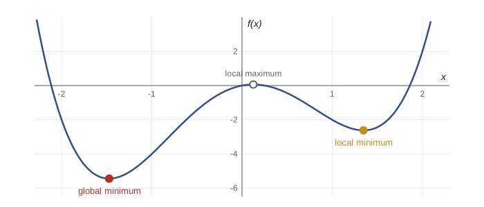
The function in the figure shows the difficulty. Its derivative \(f'(x) = 4x^3 - 8x + 1\) has three real roots, near \(-1.473\), \(0.126\) and \(1.347\). The second derivative \(f''(x) = 12x^2 - 8\) is positive at the outer two and negative at the middle one, so there are two local minima and one local maximum. Comparing values, \(f(-1.473) \approx -5.444\) while \(f(1.347) \approx -2.619\), so the global minimizer is the left one. Gradient-based methods started at \(x = 1\) slide into the right valley and stop there, perfectly satisfied with a wrong answer. Much of the power of convex optimization, the subject of lessons 9 to 11, comes from a theorem that rules this out: for a convex function every local minimizer is global.

When does a minimizer exist?

The fundamental existence result is the extreme value theorem of Karl Weierstrass. Recall that a set in \(\mathbb{R}^n\) is compact if it is closed and bounded, and that by the Bolzano–Weierstrass theorem every sequence in a compact set has a subsequence converging to a point of the set.

Theorem (Weierstrass). If \(F \subseteq \mathbb{R}^n\) is nonempty and compact and \(f : F \to \mathbb{R}\) is continuous, then \(f\) attains its minimum on \(F\).

Proof. Let \(f^* = \inf_{x \in F} f(x)\), which is either a real number or \(-\infty\). By the definition of infimum there is a sequence \(x_k \in F\) with \(f(x_k) \to f^*\) (a minimizing sequence). Since \(F\) is compact, some subsequence \(x_{k_j}\) converges to a point \(\bar x \in F\). By continuity \(f(x_{k_j}) \to f(\bar x)\). But \(f(x_{k_j})\) also tends to \(f^*\), so \(f^* = f(\bar x)\). In particular \(f^*\) is finite and \(\bar x\) is a minimizer. \(\square\)

Each hypothesis matters. On the open interval \((0, 1)\), \(f(x) = x\) has infimum 0 but no minimizer: closedness fails. On \(\mathbb{R}\), \(e^x\) has no minimizer: boundedness fails. And the function equal to \(x\) on \((0, 1]\) and to 1 at \(x = 0\) has no minimizer on \([0, 1]\): continuity fails. Since many useful feasible sets are unbounded, we also need a version for unbounded sets. A function on a closed set \(F\) is coercive if \(f(x) \to +\infty\) whenever \(\|x\| \to \infty\) within \(F\).

Corollary. If \(F\) is nonempty and closed and \(f\) is continuous and coercive on \(F\), then \(f\) attains its minimum on \(F\).

Proof. Pick any \(x_0 \in F\). By coercivity there is \(R\) such that \(f(x) > f(x_0)\) whenever \(x \in F\) and \(\|x\| > R\). The set \(F_R = \{x \in F : \|x\| \le R\}\) is closed and bounded, hence compact, and contains \(x_0\). By Weierstrass, \(f\) has a minimizer \(\bar x\) on \(F_R\), and \(f(\bar x) \le f(x_0)\). Points outside \(F_R\) have \(f(x) > f(x_0) \ge f(\bar x)\), so \(\bar x\) is a minimizer on all of \(F\). \(\square\)

The quartic \(x^4 - 4x^2 + x\) is coercive because the \(x^4\) term dominates, so it has a global minimizer, and since a minimizer of a differentiable function on \(\mathbb{R}\) must be a stationary point, comparing the stationary values finds it. This compare-the-candidates strategy is the whole of single-variable calculus optimization: list the stationary points and the boundary points, and pick the best. Linear programming turns out to have the same structure, with the vertices of a polyhedron playing the role of candidates, but there are far too many vertices to list, which is why the simplex method was such a breakthrough.

A map of problem classes

Optimization problems are classified by the form of \(f\), the \(g_i\), the \(h_j\) and \(X\), because the form determines both the theory and the algorithms. The classes below are the subject of the rest of the course.

Linear programs (LPs) have a linear objective and linear constraints: minimize \(c^Tx\) subject to \(Ax \le b\). The feasible set is a polyhedron, an intersection of finitely many half-spaces, and lessons 2 to 7 show that if an optimum exists, one occurs at a vertex. Leonid Kantorovich formulated production-planning problems of this kind in 1939 while advising a Leningrad plywood trust; George Dantzig, working on planning for the United States Air Force, proposed the general model and invented the simplex method in 1947. LPs schedule airlines, plan refinery output and route freight, and modern solvers handle millions of variables.

Integer programs (IPs) add the requirement that some variables take integer values: a plant is built or not, a truck makes 3 trips and not 2.7. This one change makes the problem dramatically harder in general, and lesson 8 introduces branch and bound, which solves integer programs by solving a tree of LPs.

Convex programs minimize a convex function over a convex set. Least squares, where one minimizes \(\|Ax - b\|^2\) as Legendre and Gauss did around 1805 to 1809, is the oldest example. Harry Markowitz's 1952 portfolio model, which minimizes the variance \(x^T\Sigma x\) of a portfolio subject to a target return, is another. Convex programs share the best property LPs have, that local optima are global, and lessons 9 to 11 build their theory.

Nonlinear programs cover everything else: nonconvex objectives, curved constraints, problems like the quartic above. Here we usually settle for local solutions and must be content with conditions, the Karush–Kuhn–Tucker conditions of lesson 11, that a local solution must satisfy.

A classic first example in the LP class is the diet problem. In 1945 the economist George Stigler asked for the cheapest combination of 77 foods that met an adult's yearly needs for nine nutrients, and by clever trial and error found a diet costing 39.93 dollars a year at 1939 prices. When the simplex method appeared, a team at the National Bureau of Standards solved Stigler's problem by hand with desk calculators and found that his heuristic answer had been only slightly above the true optimum. The diet problem is still the standard example of a blending model, and it reappears in lesson 2.

From words to a model

Much of the skill of optimization lies before any theorem is applied, in turning a description in words into a precise model. Three questions organize the work. What do we control? Those quantities become the variables, and choosing them well matters: describing a schedule by the start time of each job leads to a very different model from describing it by a yes-or-no variable for each job and time slot. What are we trying to achieve? That becomes the objective, and if there are several goals, such as low cost and low emissions, we must either weight them into one number or keep one as the objective and turn the others into constraints. What must be respected? Physical laws, budgets, capacities and logical rules become constraints.

A model is always a simplification. A linear cost ignores volume discounts, a fixed demand ignores uncertainty, and a continuous variable ignores the fact that trucks come in whole numbers. The art is to keep the model simple enough to solve and rich enough that its answer is trustworthy. A useful habit is to check units: every term in a constraint must have the same units, and an objective that adds dollars to hours is a sign that a weight is missing. Another is to test the model on a tiny instance whose answer you can see by hand before trusting it on a large one.

It also pays to ask whether the answer will be acted on directly or used to support a decision. In the first case the model must be accurate in detail; in the second, the most valuable output is often not the optimal solution itself but its sensitivity: how much the optimal cost changes if a capacity is increased or a price moves. Lesson 7 shows that linear programming delivers these marginal values, called shadow prices, essentially for free.

Computing the candidates

The program finds the global minimum of the quartic in two ways, by a coarse grid search and by locating all stationary points with a sign scan of \(f'\) followed by Newton's method, then classifies each stationary point with \(f''\). It also checks the box example and shows an infimum that is never attained.

import math

def f(x):  return x**4 - 4*x**2 + x
def df(x): return 4*x**3 - 8*x + 1
def d2f(x): return 12*x**2 - 8

# 1. coarse grid search on [-3, 3]
xs = [-3 + 6 * k / 600 for k in range(601)]
best = min(xs, key=f)
print(f"grid search: best grid point x = {best:+.3f}, f = {f(best):.4f}")

# 2. bracket sign changes of f' and polish each root with Newton's method
roots = []
for a, b in zip(xs, xs[1:]):
    if df(a) * df(b) < 0:
        x = (a + b) / 2
        for _ in range(30):
            x -= df(x) / d2f(x)
        roots.append(x)
for x in roots:
    kind = "local min" if d2f(x) > 0 else "local max"
    print(f"stationary point x = {x:+.6f}: f = {f(x):+.6f}, f'' = {d2f(x):+.3f} -> {kind}")
mins = [x for x in roots if d2f(x) > 0]
g = min(mins, key=f)
print(f"global minimum (f is coercive): x* = {g:+.6f}, f* = {f(g):.6f}")

# 3. the open box: V(x) = x (30 - 2x)^2 on the compact interval [0, 15]
V = lambda x: x * (30 - 2 * x) ** 2
cands = [0.0, 15.0, 5.0]          # endpoints and the interior root of V'
for x in cands:
    print(f"box: x = {x:4.1f} cm, V = {V(x):7.1f} cm^3")
print("largest:", max(cands, key=V), "cm cut, volume", max(V(x) for x in cands), "cm^3")

# 4. an infimum that is not attained: e^x on the real line
for x in (-1, -5, -10, -20):
    print(f"e^{x} = {math.exp(x):.3e}", end="; ")
print("inf = 0, never reached")

grid search: best grid point x = -1.470, f = -5.4441
stationary point x = -1.472998: f = -5.444192, f'' = +18.037 -> local min
stationary point x = +0.126000: f = +0.062748, f'' = -7.809 -> local max
stationary point x = +1.346997: f = -2.618556, f'' = +13.773 -> local min
global minimum (f is coercive): x* = -1.472998, f* = -5.444192
box: x =  0.0 cm, V =     0.0 cm^3
box: x = 15.0 cm, V =     0.0 cm^3
box: x =  5.0 cm, V =  2000.0 cm^3
largest: 5.0 cm cut, volume 2000.0 cm^3
e^-1 = 3.679e-01; e^-5 = 6.738e-03; e^-10 = 4.540e-05; e^-20 = 2.061e-09; inf = 0, never reached

The grid search lands within 0.003 of the true minimizer but cannot tell us how close it is, and in many dimensions a grid is hopeless: a grid of 100 points per axis in 10 dimensions has \(10^{20}\) points. The stationary-point approach is exact but relies on the problem being one-dimensional, where we can bracket every root. The rest of the course develops methods that scale: the simplex method exploits linear structure, branch and bound exploits LP relaxations, and gradient and Newton methods exploit smoothness and convexity.

How optimality is certified

A recurring theme of the course is the certificate: a short piece of evidence that proves a proposed solution is optimal, without repeating the search. For a smooth unconstrained problem, \(\nabla f(x^*) = 0\) with a positive definite Hessian certifies a local minimum. For a linear program, lesson 6 shows that a feasible solution of a related problem, the dual, certifies optimality with a single inequality check. For convex problems the Karush–Kuhn–Tucker multipliers of lesson 11 play the same role. Certificates matter in practice because solvers make rounding errors and contain bugs; a solution accompanied by a certificate can be checked independently, often in a few lines of code.

Certificates also explain why some problems are easy and others hard. An integer program can have an optimal solution with no short certificate of optimality known, and this is one face of the deep question of whether P equals NP. Linear programs, by contrast, always have short certificates when they have optimal solutions, and Leonid Khachiyan proved in 1979 that they can be solved in polynomial time. Much of the elegance of linear programming flows from this fact.