
MATH-372 · Lesson 12 of 12 · 25 min
Capstone: an optimization model for a real decision
This capstone puts the whole course to work on one decision: how a small electric utility should schedule its hydro plant, its gas plant and its purchases from the regional market over one day. The problem is a classic of operations research, studied since the early days of linear programming, because water stored behind a dam is a resource whose value depends on when it is used. We build a linear programming model, solve it exactly, read the dual solution as electricity prices and water values, check the answer with a certificate, use sensitivity analysis to price extra water, and then add an integer commitment decision for the gas plant and solve the resulting mixed-integer program. Along the way we meet, in one realistic model, vertices, degeneracy, duality, shadow prices, complementary slackness and branching.
The setting is a small utility on a river in northern Manitoba, a province that draws almost all its electricity from water. It owns one hydro station with a modest reservoir, one gas-fired unit, and a transmission tie to the regional grid, where it can buy power at prices that change through the day. The numbers below are illustrative but of realistic proportions.
The decision and the data
The day is divided into six four-hour blocks. In each block \(t\) the utility must meet a demand \(d_t\) (in MWh) from three sources: hydro generation \(h_t\), gas generation \(g_t\) and imports \(m_t\). Water is measured in the energy it can generate, MWh-equivalent, so that one unit of stored water makes one MWh. Hydro has no fuel cost; gas costs 50 dollars per MWh; imports cost \(p_t\), which follows the daily load pattern.
| Block | Hours | Demand d (MWh) | Inflow I (MWh-eq) | Import price p (dollars/MWh) |
|---|---|---|---|---|
| 1 | 0–4 | 300 | 90 | 35 |
| 2 | 4–8 | 260 | 90 | 30 |
| 3 | 8–12 | 380 | 60 | 55 |
| 4 | 12–16 | 520 | 40 | 80 |
| 5 | 16–20 | 600 | 30 | 95 |
| 6 | 20–24 | 440 | 50 | 60 |
The plant limits are: hydro output at most 480 MWh per block (120 MW), gas at most 250 MWh per block, imports at most 400 MWh per block over the tie line. The reservoir starts the day holding 900 MWh-equivalent, must stay between 600 and 1000 to respect environmental and dam-safety rules, and must end the day back at 900 or more, so that today's schedule does not borrow from tomorrow. Water may also be spilled over the dam, \(w_t \ge 0\), without generating.
The linear program
With \(S_t\) the storage at the end of block \(t\) and \(S_0 = 900\), the model is
There are 30 variables and 43 constraints besides nonnegativity. Every assumption of lesson 2 is visible and debatable. Costs are linear, ignoring the fact that a gas unit's efficiency varies with output. Hydro output is proportional to water released, ignoring the dependence of efficiency on the reservoir level (the head). Demand and prices are known in advance, ignoring forecast error. These simplifications are standard in a first planning model; each could be relaxed at the price of a harder problem, nonlinear for head effects and stochastic for uncertainty.
Before solving, some reasoning about the structure helps. Since storage must end where it started, the hydro plant can release over the day only the day's inflow, 360 MWh, plus whatever it spills. Total demand is 2500 MWh, so at least 2140 MWh must come from gas and imports. Gas at 50 dollars is cheaper than imports in blocks 3 to 6 and dearer in blocks 1 and 2. Water is free, so it should displace the most expensive source available at the time, ideally imports at 95 dollars in block 5. But the reservoir is nearly full: starting at 900 with a ceiling of 1000, the inflows of the early blocks cannot all be held until evening.
Solving and reading the solution
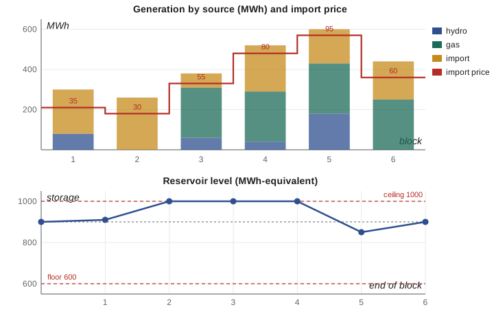
The program at the end of the lesson solves the model with the exact two-phase simplex code of lesson 6. The optimal schedule is shown below; the minimum cost is 115 300 dollars.
| Block | Hydro | Gas | Import | Spill | Storage | Marginal price | Water value |
|---|---|---|---|---|---|---|---|
| 1 | 80 | 0 | 220 | 0 | 910 | 35 | 35 |
| 2 | 0 | 0 | 260 | 0 | 1000 | 30 | 35 |
| 3 | 60 | 250 | 70 | 0 | 1000 | 55 | 55 |
| 4 | 40 | 250 | 230 | 0 | 1000 | 80 | 80 |
| 5 | 180 | 250 | 170 | 0 | 850 | 95 | 95 |
| 6 | 0 | 250 | 190 | 0 | 900 | 60 | 95 |
The schedule tells a story. Blocks 1 and 2 are cheap, so the utility imports and leaves its gas unit idle. The reservoir fills to its ceiling of 1000 by the end of block 2. In blocks 3 and 4 it is full, so every unit of inflow must be released as it arrives (60 and 40 MWh): the reservoir constraint is binding and the water cannot be saved for later. Only in block 5, the evening peak, can the plant draw the reservoir down, releasing 180 MWh, and block 6 refills it to exactly 900 with that block's inflow. Gas runs at full output from block 3 on, since it beats the import price there, and imports fill the remaining gap in every block. Note also that the early release of 80 MWh in block 1 is a consequence of the ceiling: without it, the inflows of blocks 1 and 2 would overfill the reservoir.
Prices from the dual
The dual variables of the demand constraints are the system's marginal prices: what one more MWh of demand in that block would cost. They equal the import price in every block, because imports are the marginal source everywhere, never at their 400 MWh limit. The duals of the water balance constraints are the water values: what one more MWh-equivalent of inflow in that block would save. These are the most interesting numbers in the model, and complementary slackness explains each of them.
In blocks 3 and 4 the reservoir is full, so extra inflow would have to be released at once, displacing imports at that block's price: water is worth 55 and 80. In block 5 the reservoir is between its limits and the plant is generating, so water is worth the block 5 price, 95. In block 6 the plant is not generating, but extra inflow would let the end-of-day target be met with less refill, freeing a unit of block 5 water to be released at 95, so water in block 6 is also worth 95. In block 1, water is worth 35: an extra unit cannot reach block 5, because the reservoir hits its ceiling in block 2, and the best it can do is displace a block 1 import. A water value higher than the current price is the signal to store, and lower is the signal to release; when storage is between its limits, the water value is the same in consecutive blocks, which is the economic content of complementary slackness for the storage bounds.
The dual solution is also a certificate, as in lesson 6. The program computes \(b^Ty\) for the dual vector it returns and finds exactly 115 300, the primal cost. Anyone holding the dual vector can verify optimality of the schedule by checking dual feasibility and this single equation, without trusting the solver.
Sensitivity: what is extra water worth?
Suppose a tributary can be diverted to add 10 MWh-equivalent of inflow. By lesson 7, the water value predicts the saving, provided the basis stays optimal. Added in block 1, it should save \(10 \times 35 = 350\) dollars; added in block 5, \(10 \times 95 = 950\). The program re-solves both cases and finds exactly these savings. The difference shows that timing matters more than quantity: the same water is worth almost three times as much in the evening as in the early morning, because the full reservoir in between prevents it from being carried forward.
The analysis also prices the reservoir itself. The ceiling of 1000 binds in blocks 2, 3 and 4, and its dual values are positive: raising the ceiling would let more early water be carried to the evening. A utility deciding whether to raise its dam's operating limit, or to negotiate a relaxation of an environmental constraint, would start from exactly these shadow prices, with the caution of lesson 7 that they hold only over a range.
Worked problem
Checking one water value by hand
Explain from the schedule why the water value in block 4 is 80 dollars per MWh.
Show solution
- At the end of block 4 the reservoir is at its ceiling of 1000, so one extra MWh-equivalent of inflow in block 4 cannot be stored: it must be released in block 4 or spilled.
- Hydro output in block 4 is 40 MWh, well below its 480 limit, so the extra water can be generated in block 4.
- Demand in block 4 is fixed, so the extra MWh of hydro replaces one MWh of the marginal source in block 4, imports at 80 dollars (gas is already at full output and cheaper).
- Releasing it later is impossible because the reservoir is full, and releasing it earlier is impossible because it arrives in block 4.
Answer: The extra water saves exactly one block 4 import, 80 dollars, which is the water value. The same reasoning with a reservoir that is not full gives the larger value of later blocks.
Adding a commitment decision
Real gas units cannot run at any output from zero to full. Suppose this one, when on, must produce at least 100 MWh per block, and keeping it on costs 1500 dollars per block in fixed costs (staff, auxiliary power, wear), whether or not it runs at full output. The decision to have it on in block \(t\) is a binary \(u_t \in \{0, 1\}\), and the model gains the constraints \(100u_t \le g_t \le 250u_t\) and the cost term \(1500\sum_tu_t\). This is a unit commitment problem, the mixed-integer core of every power system's day-ahead scheduling.
With six binaries there are only \(2^6 = 64\) commitment patterns, so the program simply solves the LP for each and keeps the best, a complete enumeration that is the extreme case of branch and bound with no pruning. For realistic systems with hundreds of units over 24 or 48 periods, enumeration is hopeless and branch and bound with strong LP relaxations, as in lesson 8, is the industry standard; several North American system operators moved their day-ahead market clearing from older heuristics to mixed-integer programming in the 2000s.
The best pattern runs gas only in blocks 4, 5 and 6, at full output, for a total cost of 121 050 dollars: 116 550 for energy and 4500 for commitment. The reasoning is visible in the numbers. In block 3 gas saves only \(55 - 50 = 5\) dollars per MWh, \(5 \times 250 = 1250\) dollars in all, less than the 1500 fixed cost, so the unit stays off and block 3 imports rise from 70 to 320 MWh. In blocks 4, 5 and 6 the savings of 7500, 11 250 and 2500 dollars exceed the fixed cost. A shadow price argument from the pure LP could not have revealed this, because fixed costs are invisible to marginal reasoning: it takes the integer model to see that a resource used at a small margin may not be worth switching on at all.
The whole model in code
The program builds the model from the data tables, solves it with the exact two-phase simplex solver, prints the schedule with marginal prices and water values from the dual, checks strong duality, re-solves with extra inflow in two blocks, and finally enumerates all commitment patterns for the gas unit.
from fractions import Fraction as Fr

def solve_lp(c, A, b, sense):
    """Minimize c^T x subject to rows A[i] x (sense[i] in '<=', '>=', '=') b[i], x >= 0.
    Exact two-phase simplex with Bland's rule. Returns (status, x, value, y) where y holds
    the dual values (shadow prices) of the rows: y_i = d(optimal value)/d(b_i)."""
    m, n = len(A), len(c)
    rows, rhs, cols = [], [], n
    slack = {}
    for i in range(m):                                  # add slack or surplus columns
        r = [Fr(v) for v in A[i]]
        rows.append(r); rhs.append(Fr(b[i]))
        if sense[i] != '=':
            slack[i] = cols; cols += 1
    for i in range(m):
        rows[i] += [Fr(0)] * (cols - n)
        if i in slack:
            rows[i][slack[i]] = Fr(1 if sense[i] == '<=' else -1)
        if rhs[i] < 0:                                  # make the right side nonnegative
            rows[i] = [-v for v in rows[i]]; rhs[i] = -rhs[i]
    N = cols + m                                        # artificial columns cols .. cols+m-1
    T = [rows[i] + [Fr(int(k == i)) for k in range(m)] + [rhs[i]] for i in range(m)]
    basis = [cols + i for i in range(m)]

    def price(cost):
        z = [Fr(v) for v in cost] + [Fr(0)]
        for i, j in enumerate(basis):
            z = [a - z[j] * q for a, q in zip(z, T[i])]
        return z

    def pivot(r, e):
        p = T[r][e]
        T[r] = [v / p for v in T[r]]
        for i in range(len(T)):
            if i != r and T[i][e] != 0:
                f = T[i][e]; T[i] = [a - f * q for a, q in zip(T[i], T[r])]
        basis[r] = e

    def simplex(allowed):
        while True:
            e = next((j for j in allowed if T[-1][j] < 0), None)   # Bland: smallest index
            if e is None:
                return "optimal"
            rs = [i for i in range(len(T) - 1) if T[i][e] > 0]
            if not rs:
                return "unbounded"
            t = min(T[i][-1] / T[i][e] for i in rs)
            pivot(min((i for i in rs if T[i][-1] / T[i][e] == t), key=lambda i: basis[i]), e)

    T.append(price([0] * cols + [1] * m))               # phase one
    simplex(range(N))
    if T[-1][-1] != 0:
        return "infeasible", None, None, None
    T.pop()
    for i in range(m):                                  # drive zero artificials out if possible
        if basis[i] >= cols:
            e = next((j for j in range(cols) if T[i][j] != 0), None)
            if e is not None:
                pivot(i, e)
    T.append(price(list(c) + [0] * (cols - n) + [0] * m))
    status = simplex(range(cols))                       # phase two on original columns only
    if status != "optimal":
        return status, None, None, None
    x = [Fr(0)] * N
    for i, j in enumerate(basis):
        x[j] = T[i][-1]
    # duals from B^T y = c_B, read off the artificial columns: y = c_B^T B^{-1} (sign-corrected)
    y = [-T[-1][cols + i] for i in range(m)]
    y = [(-v if Fr(b[i]) < 0 else v) for i, v in enumerate(y)]
    return "optimal", x[:n], -T[-1][-1], y
T = 6                                            # four-hour blocks of one day
demand = [300, 260, 380, 520, 600, 440]          # MWh per block
inflow = [90, 90, 60, 40, 30, 50]                # MWh-equivalent of water per block
price = [35, 30, 55, 80, 95, 60]                 # import price, dollars per MWh
GAS, GAS_CAP, IMP_CAP, HYD_CAP = 50, 250, 400, 480
S0, SMIN, SMAX, SEND = 900, 600, 1000, 900

def build(inflow=inflow, gas_on=None, gas_min=0):
    # variables per block t: h (hydro), g (gas), m (import), w (spill), S (storage at end of block)
    nv = 5 * T
    idx = lambda kind, t: 5 * t + "hgmwS".index(kind)
    c = [0] * nv
    for t in range(T):
        c[idx("g", t)] = GAS
        c[idx("m", t)] = price[t]
    rows, rhs, sense, tags = [], [], [], []
    def add(coefs, r, s, tag):
        row = [0] * nv
        for (k, t), v in coefs.items():
            row[idx(k, t)] += v
        rows.append(row); rhs.append(r); sense.append(s); tags.append(tag)
    for t in range(T):
        add({("h", t): 1, ("g", t): 1, ("m", t): 1}, demand[t], "=", ("demand", t))
        water = {("S", t): 1, ("h", t): 1, ("w", t): 1}
        if t: water[("S", t - 1)] = -1
        add(water, inflow[t] + (S0 if t == 0 else 0), "=", ("water", t))
        add({("h", t): 1}, HYD_CAP, "<=", ("hcap", t))
        cap = GAS_CAP if gas_on is None else GAS_CAP * gas_on[t]
        add({("g", t): 1}, cap, "<=", ("gcap", t))
        if gas_on is not None and gas_on[t] and gas_min:
            add({("g", t): 1}, gas_min, ">=", ("gmin", t))
        add({("m", t): 1}, IMP_CAP, "<=", ("mcap", t))
        add({("S", t): 1}, SMAX, "<=", ("smax", t))
        add({("S", t): 1}, SMIN, ">=", ("smin", t))
    add({("S", T - 1): 1}, SEND, ">=", ("send", T - 1))
    return c, rows, rhs, sense, tags, idx

c, A, b, sense, tags, idx = build()
st, x, cost, y = solve_lp(c, A, b, sense)
print(f"status {st}, minimum cost {cost} dollars")
print(" block  demand  hydro  gas  import  spill  storage  marginal price  water value")
dual = dict(zip(tags, y))
for t in range(T):
    v = lambda k: x[idx(k, t)]
    print(f"   {t + 1}    {demand[t]:5d}  {str(v('h')):>5s} {str(v('g')):>4s}  {str(v('m')):>5s}  {str(v('w')):>5s}"
          f"  {str(v('S')):>6s}   {str(dual[('demand', t)]):>8s}       {str(-dual[('water', t)]):>6s}")
print(f"hydro energy {sum(x[idx('h', t)] for t in range(T))} MWh, gas {sum(x[idx('g', t)] for t in range(T))}, "
      f"imports {sum(x[idx('m', t)] for t in range(T))}")

# certificate: the dual objective b^T y must equal the cost
print("strong duality check: b^T y =", sum(bi * yi for bi, yi in zip(b, y)), "= cost:", sum(bi * yi for bi, yi in zip(b, y)) == cost)

# sensitivity: 10 MWh more inflow in block 1, re-solved
inf2 = list(inflow); inf2[0] += 10
_, _, cost2, _ = solve_lp(*build(inf2)[:4])
print(f"10 MWh extra inflow in block 1 saves {cost - cost2} dollars "
      f"(water value {-dual[('water', 0)]} per MWh predicts {10 * -dual[('water', 0)]})")
inf3 = list(inflow); inf3[4] += 10
_, _, cost3, _ = solve_lp(*build(inf3)[:4])
print(f"10 MWh extra inflow in block 5 saves {cost - cost3} dollars (water value {-dual[('water', 4)]})")

# integer extension: the gas unit must run at least 100 MWh per block when on, and costs 1500 to keep on per block
best = None
for mask in range(2 ** T):
    on = [(mask >> t) & 1 for t in range(T)]
    cc, AA, bb, ss, _, _ = build(gas_on=on, gas_min=100)
    st, xx, cst, _ = solve_lp(cc, AA, bb, ss)
    if st == "optimal":
        total = cst + 1500 * sum(on)
        if best is None or total < best[0]:
            best = (total, on, xx)
total, on, xx = best
print(f"with commitment: gas on in blocks {[t + 1 for t in range(T) if on[t]]}, total cost {total} "
      f"(energy {total - 1500 * sum(on)} + commitment {1500 * sum(on)})")
print("   gas output by block:", [str(xx[idx('g', t)]) for t in range(T)])
print("   imports by block:   ", [str(xx[idx('m', t)]) for t in range(T)])
print(f" ({2 ** T} commitment patterns examined, each by one LP)")status optimal, minimum cost 115300 dollars block demand hydro gas import spill storage marginal price water value 1 300 80 0 220 0 910 35 35 2 260 0 0 260 0 1000 30 35 3 380 60 250 70 0 1000 55 55 4 520 40 250 230 0 1000 80 80 5 600 180 250 170 0 850 95 95 6 440 0 250 190 0 900 60 95 hydro energy 360 MWh, gas 1000, imports 1140 strong duality check: b^T y = 115300 = cost: True 10 MWh extra inflow in block 1 saves 350 dollars (water value 35 per MWh predicts 350) 10 MWh extra inflow in block 5 saves 950 dollars (water value 95) with commitment: gas on in blocks [4, 5, 6], total cost 121050 (energy 116550 + commitment 4500) gas output by block: ['0', '0', '0', '250', '250', '250'] imports by block: ['220', '260', '320', '230', '170', '190'] (64 commitment patterns examined, each by one LP)
Every number quoted in this lesson comes from this output, and the exact arithmetic means none of them carries rounding error. The model is small, but its structure, a network of storage linking periods, demand balances priced by duals and binary commitments layered on top, is the same as that of the planning models utilities and grid operators solve every day with commercial solvers and many thousands of variables.
Looking back
The capstone used nearly every idea of the course. Modelling (lesson 2) turned a description into linear constraints, including a storage balance that links periods. The fundamental theorem (lesson 3) guaranteed an optimal vertex, and the simplex method with Bland's rule and phase one (lessons 4 and 5) found it; the vertex happens to be nondegenerate, with exactly 43 positive variables and slacks for 43 rows, so its shadow prices are genuine two-sided derivatives. Duality and complementary slackness (lesson 6) gave marginal prices and water values with clear economic meanings, and a certificate of optimality. Sensitivity analysis (lesson 7) priced extra inflow and storage capacity. Integer programming (lesson 8) handled the commitment decision. Extensions would bring in the rest: hydro efficiency that depends on head makes the model nonlinear and, with suitable assumptions, convex (lessons 9 and 10), and its optimality conditions are the KKT conditions of lesson 11, whose multipliers would again be water values. For the managerial side of such models, including forecasting, capacity and supply chains, see MBA-513 Operations and Supply Chain Management; for the search and learning algorithms that rest on the methods of lessons 8 and 10, see CMPUT-366 Artificial Intelligence and CMPUT-466 Deep Learning.
Common mistakes
MistakeLetting the reservoir end the day empty.
InsteadWithout an end-of-horizon storage target, the model spends tomorrow's water today; require \(S_6 \ge S_0\) or value end storage.
MistakeReading a water value as the price in the block where the water arrives.
InsteadWater value reflects where the water can best be used; with free storage it equals the price of a later block.
MistakeExpecting shadow prices to reveal whether a unit should be switched on.
InsteadFixed commitment costs are invisible to marginal analysis; they need integer variables.
MistakeForgetting spill variables.
InsteadWithout spill, a full reservoir with high inflow can make the model infeasible.
MistakeTreating the model's optimal schedule as exact for a real utility.
InsteadThe model is a simplification; use its prices and sensitivities as guidance and re-solve as forecasts change.
Summary and key terms
- A hydro-thermal dispatch model has demand balances, water balances linking periods, reservoir bounds and an end-of-day storage target.
- The optimal schedule uses imports in cheap blocks, gas when it is cheaper than imports, and stored water at the evening peak, subject to the reservoir ceiling.
- Duals of the demand constraints are marginal prices; duals of the water balances are water values.
- Water values depend on timing: 35 dollars per MWh in block 1 but 95 in blocks 5 and 6, because the full reservoir blocks carrying early water forward.
- Re-solving with extra inflow confirms the water values as exact sensitivities within their ranges.
- A unit commitment extension with binary on/off decisions changes the schedule in a way no marginal analysis predicts.
- hydro-thermal dispatch
- Scheduling hydro and thermal generation to meet demand at least cost.
- water value
- The marginal value of one more unit of stored water, the dual of the water balance.
- marginal price
- The cost of serving one more unit of demand, the dual of the demand constraint.
- spill
- Water released without generating electricity.
- unit commitment
- The mixed-integer problem of deciding which generating units are on in each period.
- end-of-horizon condition
- A constraint or value on final storage that prevents the model from exhausting resources at the end.
Practice problems
Work each problem on paper first, then reveal the answer to check.
Without solving, explain why gas does not run in blocks 1 and 2 of the LP.
Show answer
Imports cost 35 and 30 dollars there, less than gas at 50, and the tie line has room (220 and 260 of 400 MWh), so gas is never the cheapest source.
If the end-of-day target were 800 instead of 900, how much could the optimal cost fall, at most to first order?
Show answer
The extra 100 MWh of water could be released in block 5 at 95 dollars; the dual of the end constraint is about 95, so roughly 9500 dollars, if the basis stays optimal over that range.
Why are the marginal prices equal to the import prices in every block?
Show answer
Imports are the marginal source in every block and never hit their limit, so one more MWh of demand is one more MWh imported.
Suppose the reservoir ceiling were 1200. Would the water value in block 1 rise or fall? Explain.
Show answer
Rise: with more room, early inflow could be stored until block 5 and displace 95-dollar imports instead of 35-dollar ones.
Write the constraints that make gas output either zero or between 100 and 250 MWh in block \(t\).
Show answer
\(100u_t \le g_t \le 250u_t\), with \(u_t \in \{0, 1\}\).
In the commitment model, why is gas off in block 3 but on in block 6?
Show answer
Saving per MWh is 5 dollars in block 3 (1250 in all, below the 1500 fixed cost) but 10 dollars in block 6 (2500 in all, above it).
Lesson quiz · 5 questions
Score 60% or more to complete this lesson.
Create a free account to save your progress, take quizzes and earn a certificate.