The CMOS inverter

The CX-1 digital half is small by modern standards: four 24-bit period counters, a register file, a serial interface and some control logic, perhaps five thousand gates. It will be synthesized from the foundry's standard cell library, and Amara will never draw most of those gates by hand. But every one of them is built on the CMOS inverter, and the inverter is where the speed, power and noise behaviour of digital CMOS can be understood from first principles. This lesson derives the inverter's static transfer characteristic, its noise margins, its switching speed and its power dissipation, using the transistor models of lesson 3.

How the inverter works

A CMOS inverter is one NMOS and one PMOS transistor with their gates tied together as the input and their drains tied together as the output. The NMOS source goes to ground and the PMOS source to the supply V_DD. With the input low, the NMOS is off and the PMOS is on, pulling the output to V_DD; with the input high, the NMOS is on and the PMOS off, pulling the output to ground. In either steady state one device is off, so no current flows from supply to ground apart from leakage. This is the property that made CMOS the dominant logic family: a gate that is not switching consumes almost no power.

The output also reaches the full supply rails, because the on transistor has no current to carry once the load capacitance is charged and so drops no voltage. Logic levels are restored at every gate: a slightly degraded input produces a clean output. And the input draws no static current, so one gate can drive many others. These three properties, zero static power, rail-to-rail outputs and regenerative levels, are what lesson 5 relies on when it builds more complex gates from the same two-network structure.

The voltage transfer characteristic

The voltage transfer characteristic (VTC) plots the output voltage against the input as the input is swept slowly from 0 to V_DD. At each input voltage the output settles where the NMOS and PMOS currents are equal, because no current can go anywhere else. Finding that point is a one-variable root-finding problem, and the lesson's code solves it by bisection with the square-law models of lesson 3, including channel-length modulation, for an inverter with a 0.5 µm NMOS and a 1.5 µm PMOS at the minimum 0.18 µm length on a 1.8 V supply.

# CMOS inverter on the illustrative 180 nm process: VDD = 1.8 V, square law with lambda
VDD = 1.8
kn, kp = 300e-6, 75e-6          # mu Cox, A/V^2
VTN, VTP = 0.45, 0.45           # magnitudes
lam = 0.1                       # channel-length modulation at minimum length, 1/V
Wn, Wp, L = 0.5, 1.5, 0.18      # um

def ids_n(vgs, vds):
    b = kn * Wn / L
    if vgs <= VTN: return 0.0
    vov = vgs - VTN
    if vds < vov: return b * (vov - vds / 2) * vds * (1 + lam * vds)
    return 0.5 * b * vov ** 2 * (1 + lam * vds)

def ids_p(vsg, vsd):
    b = kp * Wp / L
    if vsg <= VTP: return 0.0
    vov = vsg - VTP
    if vsd < vov: return b * (vov - vsd / 2) * vsd * (1 + lam * vsd)
    return 0.5 * b * vov ** 2 * (1 + lam * vsd)

def vout(vin):
    lo, hi = 0.0, VDD                # bisection on the output node current balance
    for _ in range(60):
        vo = (lo + hi) / 2
        if ids_p(VDD - vin, VDD - vo) > ids_n(vin, vo): lo = vo
        else: hi = vo
    return (lo + hi) / 2

pts = [(i * VDD / 1800, vout(i * VDD / 1800)) for i in range(1801)]
vm = min(pts, key=lambda p: abs(p[0] - p[1]))[0]
gains = [(pts[i][0], (pts[i + 1][1] - pts[i - 1][1]) / (pts[i + 1][0] - pts[i - 1][0])) for i in range(1, 1800)]
vil = next(v for v, g in gains if g < -1)
vih = next(v for v, g in reversed(gains) if g < -1)
voh, vol = vout(vil), vout(vih)
gmax = min(g for v, g in gains)
print(f"switching threshold VM = {vm:.3f} V")
print(f"VIL = {vil:.3f} V (VOH = {voh:.3f} V), VIH = {vih:.3f} V (VOL = {vol:.3f} V)")
print(f"noise margins NML = {vil - vol:.3f} V, NMH = {voh - vih:.3f} V; peak gain {gmax:.1f}")

# Propagation delay estimate with an average on-resistance, and power
c_load = 10e-15                    # fan-out plus wire, F
i_n = 0.5 * kn * Wn / L * (VDD - VTN) ** 2
i_p = 0.5 * kp * Wp / L * (VDD - VTP) ** 2
t_phl = c_load * (VDD / 2) / i_n
t_plh = c_load * (VDD / 2) / i_p
print(f"saturation currents: n {i_n * 1e6:.0f} uA, p {i_p * 1e6:.0f} uA")
print(f"tPHL ~ {t_phl * 1e12:.1f} ps, tPLH ~ {t_plh * 1e12:.1f} ps (constant-current estimate)")
alpha, f = 0.15, 20e6
print(f"dynamic power per gate at a = {alpha}, f = 20 MHz: {alpha * c_load * VDD ** 2 * f * 1e9:.2f} nW")

switching threshold VM = 0.868 V
VIL = 0.727 V (VOH = 1.696 V), VIH = 0.988 V (VOL = 0.119 V)
noise margins NML = 0.608 V, NMH = 0.708 V; peak gain -48.8
saturation currents: n 759 uA, p 570 uA
tPHL ~ 11.9 ps, tPLH ~ 15.8 ps (constant-current estimate)
dynamic power per gate at a = 0.15, f = 20 MHz: 97.20 nW

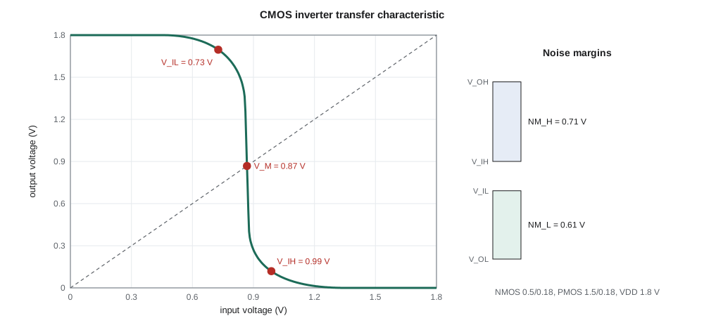
The curve has the familiar shape. For inputs below the NMOS threshold the output sits at V_DD; as the input rises the NMOS begins to conduct and the output sags slightly; near the middle both transistors are saturated and the output falls steeply; and above V_DD − |V_TP| the PMOS is off and the output sits at ground. The steep region is where the inverter acts as a high-gain amplifier, with a peak gain of nearly 50 here, set by the transistors' output resistances.

The switching threshold V_M is the input voltage at which the output equals the input, where the curve crosses the 45° line. Setting the two saturation currents equal gives V_M in closed form. With matched thresholds and the ratio r = √(k_p/k_n), where each k includes W/L, it depends only on the device ratio.

The test inverter has a PMOS three times as wide as its NMOS, but the PMOS has only a quarter of the NMOS's μCox, so k_p/k_n = 0.75 and r ≈ 0.87. The formula gives V_M ≈ (0.45 + 0.87 × 1.35)/1.87 ≈ 0.87 V, matching the simulation's 0.868 V, a little below the midpoint of 0.9 V. To centre V_M exactly the PMOS would need to be four times the NMOS width. Standard cell libraries usually choose a ratio of two to three rather than four, accepting a slightly low threshold to save area and input capacitance.

Noise margins

Noise margins say how much noise a logic signal can tolerate before a gate misreads it. They are defined from the two points on the VTC where the slope is −1. Below V_IL the inverter's gain is less than one, so small input disturbances are attenuated; above V_IH the same holds on the other side. The low noise margin NM_L = V_IL − V_OL is how much a valid low output can be raised by noise and still be read as low by the next gate; the high noise margin NM_H = V_OH − V_IH is the same for a high.

For the test inverter the code finds V_IL = 0.73 V and V_IH = 0.99 V, giving NM_L of about 0.61 V and NM_H of about 0.71 V, a third or more of the supply each. Those margins are generous, and they explain why digital CMOS tolerates the supply bounce and crosstalk of a busy chip. They also show what happens if the threshold moves: a process corner that strengthens the NMOS lowers V_M and shrinks NM_L. A designer checks noise margins across corners for any custom gate, and the library vendor has already done so for standard cells.

Switching speed

A gate's delay is the time it takes to charge or discharge the capacitance at its output: the drain capacitances of its own transistors, the wiring, and the gate capacitance of every input it drives. Propagation delay is conventionally measured from the 50 % point of the input to the 50 % point of the output. Two simple estimates bracket the result.

The constant-current estimate assumes the switching transistor delivers its saturation current throughout the transition, so the delay is the charge C V_DD/2 divided by that current. The code gives about 12 ps for the falling output and 16 ps for the rising output into 10 fF. It is optimistic, because the device leaves saturation as the output approaches the rail and because the square law overestimates short-channel current. The RC estimate replaces each on transistor by an effective resistance R_eff, roughly V_DD divided by its average current, and uses t_p ≈ 0.69 R_eff C. For a minimum NMOS in a 180 nm process R_eff is about 10 kΩ·µm divided by width, so a 0.5 µm device is about 20 kΩ, and into 10 fF the falling delay is about 0.69 × 20 kΩ × 10 fF ≈ 140 ps. The truth for this process is in between, close to 60 to 80 ps, which is what a simulation with the foundry models gives.

The RC model is the more useful of the two, because it scales correctly. Widening a transistor by a factor k divides its resistance by k but multiplies its own drain and gate capacitance by k. When the load is dominated by other gates, widening speeds the gate up; when it is dominated by the gate's own parasitics, it does not. Lesson 5 turns that observation into the method of logical effort, which sizes whole paths of gates for minimum delay.

A convenient process-independent unit of speed is the delay of an inverter driving four copies of itself, the fan-out-of-four or FO4 delay. For a 180 nm process the FO4 delay is about 70 to 90 ps; for modern nodes it is under 10 ps. A rule of thumb that has held for decades is that a well-designed synchronous chip has a clock period of roughly 15 to 25 FO4 delays, so a 180 nm design is comfortable up to a few hundred megahertz. CX-1's 20 MHz clock, a period of 50 ns or over 500 FO4 delays, is easy, which is why lesson 6 concentrates on power and hold time rather than setup time.

Power dissipation

A CMOS gate dissipates power in three ways. Dynamic power is the energy spent charging and discharging the load capacitance. Each time the output rises, C_L V_DD² of energy is drawn from the supply: half is stored on the capacitor and half is lost in the PMOS; when the output falls, the stored half is lost in the NMOS. If a node switches from low to high with probability α each clock cycle, the average power is α C_L V_DD² f. Short-circuit power flows during each transition while both devices are briefly on; it is usually a tenth or less of the dynamic power if input edges are reasonably fast. Static power is leakage: subthreshold current through off transistors, junction leakage and gate tunnelling. In a 180 nm process static power is small at room temperature but grows rapidly with temperature, as lesson 6 shows.

The test inverter, loaded with 10 fF and toggling with α = 0.15 at 20 MHz, dissipates about 97 nW. Five thousand such gates would dissipate about half a milliwatt, small next to the analog blocks. The equation's V_DD² explains why digital logic runs on the 1.8 V core supply rather than the 3.3 V I/O supply: the same logic at 3.3 V would dissipate more than three times the power. It also explains the long history of supply scaling in digital design and the techniques of lesson 6, which reduce α and f where they can.

Sizing the inverter in a library

Standard cell libraries offer each logic function in several drive strengths, labelled ×1, ×2, ×4 and so on, which are the same circuit with wider transistors. A synthesis tool picks the smallest drive that meets timing, because larger cells cost area and input capacitance and load the gate before them. Libraries also include buffers and inverters in strengths up to ×16 or ×32 for long wires and large fan-outs, and they characterize every cell's delay and power as functions of input slew and output load in tables that the timing tools interpolate. When Amara reads a timing report for the CX-1 counters, each line is one of those table lookups.

A full-custom designer can also use ratios that the library does not offer. The CX-1 comparator's output stage, for example, uses an inverter deliberately skewed with a weak NMOS and strong PMOS, so that its switching threshold is high, about 1.1 V, and it ignores small dips on its input. The same VTC calculation, with different widths, predicts the shift.