MOSFET models for IC design

Every analog decision on CX-1 begins with a transistor model, and the model a designer uses by hand is very different from the model the simulator uses. The foundry's simulation models, of the BSIM family for a process like this one, have hundreds of parameters and describe the device accurately across every bias, size and temperature. They are indispensable for verification and useless for design, because they do not tell a designer which width to choose. Hand design needs a model simple enough to solve in one's head and accurate enough to land close to the final answer. This lesson reviews the square-law model, shows where it fails in a modern process, and introduces the gm/ID method that Priya uses to size every analog transistor on CX-1.

The square-law model and its parameters

ELE-240 introduced the long-channel model of an enhancement MOSFET. With the gate-source voltage above threshold by the overdrive V_ov = V_GS − V_T and the drain-source voltage beyond V_ov, the device is in saturation and the drain current is set by the overdrive, with a small increase with drain voltage from channel-length modulation. Below V_DS = V_ov the device is in the triode region and acts like a voltage-controlled resistor.

The process parameters for the illustrative CX-1 process are μnCox = 300 µA/V² for NMOS and μpCox = 75 µA/V² for PMOS, so a PMOS device needs about four times the width of an NMOS device to carry the same current at the same overdrive. Threshold voltages are about 0.45 V for both types. Channel-length modulation is best described not by a fixed λ but by its dependence on length: λ is roughly inversely proportional to L, so the product λL is approximately a process constant, about 0.04 µm/V here. Doubling a transistor's length at the same current doubles its output resistance. That single fact explains why analog transistors on CX-1 are drawn at 0.5 to 2 µm long while digital transistors are drawn at the 0.18 µm minimum.

The quantity that matters most to an analog designer is the intrinsic gain of a single transistor, g_m r_o, the largest voltage gain one device can give with an ideal current-source load. From the square law it is 2/(λ V_ov), which favours low overdrive and long channels. At V_ov = 0.2 V and L = 1 µm, λ is 0.04 V⁻¹ and g_m r_o is 250. At minimum length the same device gives about 45. Intrinsic gain has fallen steadily with each process generation, which is one reason analog circuits stay in older nodes.

The body effect

The threshold voltage depends on the voltage between the source and the body. When the source of an NMOS device rises above the substrate, as it does in a source follower or the upper device of a cascode, the depletion region under the channel widens, more gate voltage is needed to form the channel, and V_T rises.

For the illustrative process γ is about 0.45 V^½ and 2φ_F about 0.8 V. With 0.5 V between source and body, the threshold rises from 0.45 V to about 0.56 V; with 1 V, to about 0.65 V. In a 1.8 V circuit, a 200 mV loss of headroom can decide whether a cascode works at all. The body effect also adds a second transconductance, g_mb, through which the body acts as a back gate, typically 0.15 to 0.25 times g_m. NMOS devices in this process share the grounded substrate, so their body effect cannot be avoided. PMOS devices sit in their own n-wells, and a designer can tie each well to its device's source to remove the body effect, at the cost of area for separate wells.

Where the square law fails

The square law was derived for long channels and strong inversion, and a 180 nm process violates both assumptions in ways that matter. Three effects are worth knowing by name.

Velocity saturation limits the speed of carriers in the high lateral fields of a short channel. Instead of rising with the square of the overdrive, the drain current of a minimum-length device rises nearly linearly once the overdrive exceeds a few hundred millivolts. The square law can overestimate the saturation current of a minimum-length digital transistor by a factor of two, which is why lesson 4 uses it only for rough delay estimates. Analog devices drawn at 0.5 µm or more, biased at small overdrives, are much less affected.

Mobility degradation from the vertical field of the gate reduces the current at high gate voltages, with a similar effect.

Weak inversion is the most important for low-power design. Below threshold the drain current does not vanish as the square law predicts; it falls exponentially with decreasing gate voltage, in the same way as a bipolar transistor's collector current depends on its base-emitter voltage, but with a slope factor n of about 1.3 to 1.5. Many low-power analog circuits, including much of CX-1, deliberately operate with small overdrives near this region, called moderate inversion, where neither the square law nor the exponential law is accurate.

The gm/ID method

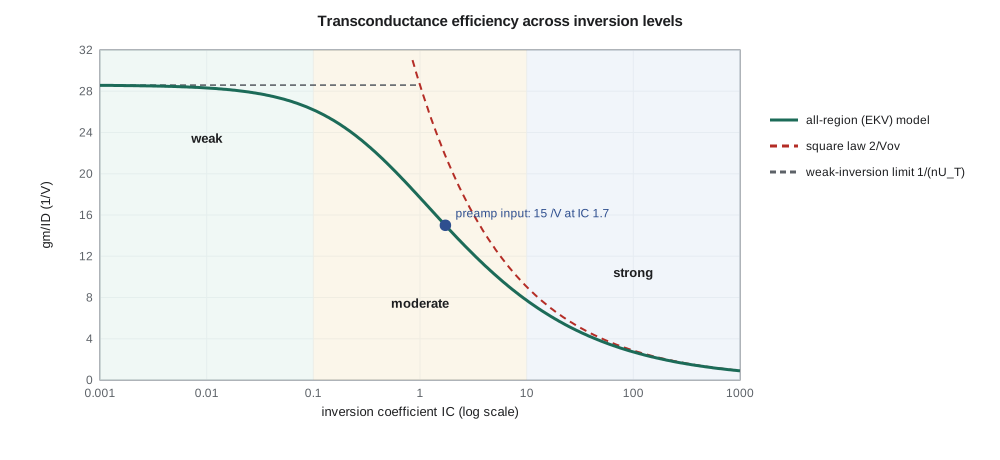
The gm/ID method replaces the question “what overdrive should this transistor have?” with a better one: “how much transconductance should each microampere of bias current buy?” The ratio g_m/I_D is called the transconductance efficiency. It is large, near its maximum of 1/(nU_T) or about 28 V⁻¹, in weak inversion, where the device is efficient but slow and large. It is small in strong inversion, where the square law gives 2/V_ov, and the device is fast and compact but needs more current for the same g_m. The designer picks g_m/I_D for each device to balance power, speed, area, matching and swing, and the method then gives the width.

The method works because g_m/I_D depends on the inversion level of the device rather than on its absolute size. A useful way to state the inversion level is the inversion coefficient IC, the ratio of the drain current to a specific current I_spec that scales with W/L. An IC of 0.1 or less is weak inversion; an IC of 10 or more is strong inversion; between them is moderate inversion. The EKV model, developed in the 1990s, gives a single smooth expression that is accurate in all three regions.

In practice a designer does not trust a formula for the final sizes. Priya's team sweeps the foundry's simulation models once, for each device type and several lengths, and tabulates g_m/I_D, the current density I_D/W, the transit frequency f_T and the intrinsic gain g_m r_o against g_m/I_D. Design then becomes a matter of reading tables rather than solving equations, and the tables carry the full accuracy of the simulation models. The interpolation formula above is what the lesson's code uses in place of those tables, and it is close enough to show the method.

import math
# MOSFET models on the illustrative 180 nm process: NMOS, 27 C
UT = 0.0259          # thermal voltage kT/q, V
n = 1.35             # subthreshold slope factor
kn = 300e-6          # mu_n Cox, A/V^2
VT0, gamma, phi2 = 0.45, 0.45, 0.80

def vt(vsb):
    return VT0 + gamma * (math.sqrt(phi2 + vsb) - math.sqrt(phi2))

def gm_id(ic):
    """EKV-style interpolation of gm/ID across weak, moderate and strong inversion."""
    return 2.0 / (n * UT * (1.0 + math.sqrt(1.0 + 4.0 * ic)))

def ispec(w_over_l):
    return 2.0 * n * kn * UT ** 2 * w_over_l

print("body effect: VT =", ", ".join(f"{vt(v):.3f} V at VSB {v} V" for v in (0, 0.5, 1.0)))
print(f"unit specific current I_spec (W/L = 1) = {ispec(1) * 1e9:.0f} nA")
print(" IC     gm/ID (1/V)   square law 2/Vov   region")
for ic in (0.01, 0.1, 1, 10, 100):
    g = gm_id(ic)
    vov = 2 * n * UT * math.sqrt(ic)              # strong-inversion estimate
    sq = 2 / vov
    region = "weak" if ic <= 0.1 else ("moderate" if ic < 10 else "strong")
    print(f"{ic:>6}  {g:8.1f}      {sq:8.1f}        {region}")

# Size an input device: gm = 150 uS from 10 uA, L = 0.5 um
gm, i_d, L = 150e-6, 10e-6, 0.5
target = gm / i_d
# solve gm_id(ic) = target for ic
lo, hi = 1e-4, 1e4
for _ in range(100):
    mid = math.sqrt(lo * hi)
    if gm_id(mid) > target: lo = mid
    else: hi = mid
ic = lo
wl = i_d / (ic * ispec(1))
print(f"gm/ID = {target:.0f} /V needs IC = {ic:.2f}; W/L = {wl:.1f}; W = {wl * L:.1f} um at L = {L} um")
vov = 2 * n * UT * math.sqrt(ic)
print(f"overdrive estimate {vov * 1e3:.0f} mV, VDSsat about {max(vov, 4 * UT) * 1e3:.0f} mV")

body effect: VT = 0.450 V at VSB 0 V, 0.561 V at VSB 0.5 V, 0.651 V at VSB 1.0 V
unit specific current I_spec (W/L = 1) = 543 nA
 IC     gm/ID (1/V)   square law 2/Vov   region
  0.01      28.3         286.0        weak
   0.1      26.2          90.4        weak
     1      17.7          28.6        moderate
    10       7.7           9.0        strong
   100       2.7           2.9        strong
gm/ID = 15 /V needs IC = 1.73; W/L = 10.6; W = 5.3 um at L = 0.5 um
overdrive estimate 92 mV, VDSsat about 104 mV

The table shows the square law's failure plainly. At an inversion coefficient of 1, in the middle of moderate inversion, the square law predicts g_m/I_D of 28.6 V⁻¹, more than half again the true value of 17.7 V⁻¹. A circuit designed with the square law at that bias would have far less gain and bandwidth than expected. Only above IC = 10 do the two agree within about fifteen percent.

The sizing example at the end is the pattern for the rest of the course. The CX-1 preamplifier needs an input transistor with 150 µS of transconductance from 10 µA. That fixes g_m/I_D at 15 V⁻¹, which the curve places at an inversion coefficient of about 1.7, comfortably in moderate inversion. The specific current then gives W/L of about 10.6, and with L = 0.5 µm chosen for gain, the width is 5.3 µm. The effective overdrive of about 90 mV and the saturation voltage of about 100 mV tell the designer how much headroom the device needs.

That example captures the most useful rule of thumb in analog IC design. Devices whose job is to convert voltage into current efficiently, such as amplifier inputs, want high g_m/I_D, from about 15 to 25 V⁻¹. Devices whose job is to carry a precise current, such as mirrors and current sources, want low g_m/I_D, from about 5 to 10 V⁻¹, so that their threshold mismatch matters less and they have more output resistance. Devices that must be fast, such as those in high-frequency paths, also want low g_m/I_D, because the transit frequency f_T rises with overdrive.

Capacitances and the transit frequency

A transistor's speed is set by its capacitances. In saturation the gate-source capacitance is about two thirds of the gate area times Cox, plus an overlap term at each edge; the gate-drain capacitance is mainly overlap; and the source and drain each have junction capacitance to the body that depends on their area and perimeter. The transit frequency, the frequency at which the current gain of a device with a shorted drain falls to one, is f_T = g_m/(2π(C_gs + C_gd)). It rises with overdrive and falls with the square of length, which is why the long devices that give analog circuits their gain are also slow.

For the preamplifier input device sized above, C_gs is about two thirds of 5.3 µm × 0.5 µm × 8.6 fF/µm², or 15 fF, plus overlap of about 2 fF, so f_T is about 150 µS/(2π × 17 fF), roughly 1.4 GHz. That is far above the 5 MHz bandwidth CX-1 needs, which tells Priya she could lengthen the device further for gain and matching without running out of speed. On a minimum-length digital transistor at full overdrive, f_T approaches the tens of gigahertz that make the 180 nm process useful for radio work too.

Temperature

Two temperature effects pull in opposite directions. The threshold voltage falls by about 1 to 2 mV per kelvin as temperature rises, which increases the current at a fixed gate voltage. Mobility falls roughly as T^{−1.5}, which decreases it. At high overdrives mobility wins and the current falls with temperature; at low overdrives the threshold wins and the current rises. Between them is a temperature-independent bias point, often used in references. For CX-1, which must work from −40 °C to 85 °C in a signal cabinet and up to 125 °C at the junction near a hot speaker driver, every analog block is simulated across the full range, and lesson 8 designs bias currents that track temperature in a controlled way.