
ELE-445 · Lesson 12 of 12 · 24 min
Design review, verification and tape-out
Five months after Daniel's question, every CX-1 block has a schematic, a layout and a stack of simulation results. The chip is assembled: 5.76 mm² of silicon, 32 pads, the analog blocks at one end and the counters and serial interface at the other. A shared wafer run closes in three weeks. Before the layout database goes to the foundry, the team holds the review that Daniel's rule demands. Its question is simple and its answer is not: is there any reason to believe this chip will not work? This lesson follows the review, covering what verification across process, voltage and temperature means, how Monte Carlo analysis predicts yield, why trim and test structures go on a first chip, how electrostatic discharge and latch-up are prevented, and what the tape-out checklist contains.
What verification has to cover
A chip that works at the typical corner, at 1.8 V and 27 °C, in simulation, has passed the easiest test it will ever face. Production parts will come from every corner of the process window, run from supplies that sag and ripple, and sit in cabinets from −40 °C to 85 °C ambient, with their junctions hotter. Verification must therefore cover the whole space, and it does so in three ways. Corner simulation runs each block at the extreme process corners of lesson 2, SS, FF, SF and FS for the transistors and high and low corners for the resistors and capacitors, at the supply and temperature extremes. Monte Carlo simulation draws random values for the global and local variation of every device, many hundreds of times, and builds distributions of each performance measure. Mixed-signal simulation runs the analog blocks at transistor level together with a model of the digital logic, to check that the two halves work together: that the converter's control logic sequences the capacitor switches correctly, that the counters gate their clocks when they should, and that the serial interface can read and write every register.
Priya's design record shows each block's results laid out against its specification. The review goes through them block by block.
The op-amp across corners
The two-stage op-amp of lesson 10 is the first test of the bias strategy of lesson 8. Its GBW depends on g_m1/C_c, and the constant-gm bias makes g_m1 proportional to 1/R, so the GBW should track 1/(RC) rather than the transistors. Its phase margin depends on the ratio of the GBW to the non-dominant poles, which the nulling resistor, made from the same poly as the bias resistor, should keep stable.
import math, random
random.seed(2026)
# Monte Carlo of the CX-1 analog front end: preamp offset, bandgap output and op-amp GBW
N = 5000
sig_os = 1.17e-3          # preamp input offset sigma from lesson 9, V
spec_os = 4.0e-3          # data-sheet limit, V
vref_nom, sig_vref = 1.2955, 0.012     # untrimmed bandgap: sigma about 0.9 %
trim_step = 0.004         # 4-bit trim, 4 mV steps, +-32 mV range
gbw_nom = 5.0e6

fails_os = sum(1 for _ in range(N) if abs(random.gauss(0, sig_os)) > spec_os)
print(f"offset: {fails_os} of {N} exceed {spec_os * 1e3:.0f} mV -> yield {1 - fails_os / N:.4f}")
print(f"  analytic: |x| > {spec_os / sig_os:.2f} sigma -> {math.erfc(spec_os / sig_os / math.sqrt(2)):.5f} fail")

untrim_ok = trim_ok = 0
for _ in range(N):
    v = vref_nom + random.gauss(0, sig_vref)
    if abs(v - 1.2955) <= 0.010: untrim_ok += 1
    code = max(-8, min(7, round((1.2955 - v) / trim_step)))
    vt = v + code * trim_step
    if abs(vt - 1.2955) <= 0.003: trim_ok += 1
print(f"bandgap within 10 mV untrimmed: {untrim_ok / N:.3f}; within 3 mV after trim: {trim_ok / N:.3f}")

# Corners for the two-stage op-amp of lesson 10, biased by a constant-gm cell (gm ~ 1/R)
def opamp(mos, rf, cf, t):
    rt = rf * (1 - 1.0e-3 * (t - 27))            # poly resistor: corner factor and -1000 ppm/K
    gbw = 5.0e6 / (rt * cf)                     # gm1/Cc with gm1 ~ 1/R
    p_mirror = 60e6 * mos * ((t + 273.15) / 300.15) ** -1.5
    p4 = 48e6 / rt                              # Rz C1 pole; Rz is the same poly as the bias resistor
    pm = 90 - math.degrees(math.atan(gbw / p_mirror)) - math.degrees(math.atan(gbw / p4))
    return gbw, pm
cases = [("TT, R typ, C typ", 1.00, 1.0, 1.0), ("SS, R low, C low", 0.85, 0.8, 0.9),
         ("FF, R high, C high", 1.15, 1.2, 1.1), ("SS, R high, C high", 0.85, 1.2, 1.1)]
print("case                  temp   GBW (MHz)   PM (deg)")
for name, mos, rf, cf in cases:
    for t in (-40, 27, 125):
        g, pm = opamp(mos, rf, cf, t)
print(f" {name:<20} {t:>4} {g / 1e6:5.2f} {pm:5.1f}")offset: 3 of 5000 exceed 4 mV -> yield 0.9994 analytic: |x| > 3.42 sigma -> 0.00063 fail bandgap within 10 mV untrimmed: 0.598; within 3 mV after trim: 0.994 case temp GBW (MHz) PM (deg) TT, R typ, C typ -40 4.69 81.0 TT, R typ, C typ 27 5.00 79.3 TT, R typ, C typ 125 5.54 76.0 SS, R low, C low -40 6.51 78.4 SS, R low, C low 27 6.94 75.6 SS, R low, C low 125 7.70 70.4 FF, R high, C high -40 3.55 82.6 FF, R high, C high 27 3.79 81.4 FF, R high, C high 125 4.20 79.3 SS, R high, C high -40 3.55 81.9 SS, R high, C high 27 3.79 80.3 SS, R high, C high 125 4.20 77.4
The corner table bears the strategy out. The GBW ranges from 3.6 MHz, with high resistance and high capacitance at −40 °C, to 7.7 MHz, with low resistance and low capacitance at 125 °C. That 2:1 range comes entirely from the passive components, and the transistor corner barely matters: the SS and FF rows with the same resistor and capacitor corners are identical in GBW. The phase margin stays between 70° and 83° everywhere, because the cancelling zero moves with the second pole. The worst case, 70° at the low-resistance corner with slow transistors at 125 °C, is where the GBW is highest and the mirror pole lowest, and it still clears the 60° requirement. Daniel asks what the preamplifier's closed-loop bandwidth does at the 3.6 MHz corner: at a gain of 30 it falls to about 120 kHz, still thirty times the voice band. The op-amp passes.
Monte Carlo and yield
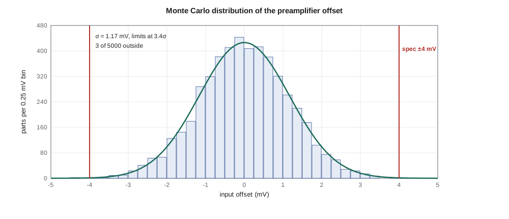
Corners bound the global variation but say nothing about local mismatch, which Monte Carlo analysis covers. Each run draws random threshold and current-factor offsets for every transistor, scaled by Pelgrom's law to its area, and random values for the global parameters. The preamplifier offset from lesson 9, after Priya enlarged its load, has σ of about 0.9 mV in her simulation; the review uses the more conservative 1.17 mV of the original design to see how much margin there is. Against the 4 mV specification, three parts in 5 000 fail, a yield of 99.94 %, consistent with the analytic tail probability of a normal distribution beyond 3.4σ.
A specification at 3σ fails about one part in 370 for that measure alone; a chip with twenty independent 3σ specifications would lose about five percent of its parts. Production chips are therefore designed so that each specification sits at four to six sigma, and the product's data sheet limits are set from characterization of many real parts rather than from the design targets. Daniel asks that every CX-1 specification be shown at its sigma level in the design record, so that the weakest ones are obvious.
Trim
Some quantities cannot be designed to their specification and must be trimmed. The bandgap of lesson 8 is the CX-1 example. Its untrimmed spread, dominated by the op-amp offset multiplied by the PTAT gain, has a σ of about 12 mV, so only about 60 % of parts fall within 10 mV of nominal. A 4-bit trim, a resistor tap selected by a code from −8 to +7 in 4 mV steps, is set at production test: the tester measures each part's reference, computes the code and writes it into a small one-time-programmable memory. After trim, 99.4 % of parts are within 3 mV. The few that remain outside have spreads beyond the trim range and are rejected at test.
Trim has costs: the programmable memory or fuses, a test-time step and a test program that must be right. It also needs the trim network to be designed so that the steps are monotonic and the range covers the spread with margin. Priya adds a second trim, for the bias current, with the same mechanism, so that the comparator's speed and the op-amp's GBW can be centred if the first silicon shows the resistor value far from the model.
Electrostatic discharge protection
A chip is most at risk before it is ever powered: when it is handled during assembly, test and board manufacture. A person can carry several kilovolts of static charge, and the human-body model used for qualification represents that discharge as about 100 pF through 1.5 kΩ into a pin, a pulse of an ampere or more lasting about a hundred nanoseconds. The 4 nm gate oxide of a core transistor breaks down at well under 10 V. Without protection, a single touch would destroy the chip.
Every pin therefore has an electrostatic discharge (ESD) protection network that gives the discharge current a safe path to a supply rail, clamping the pin voltage below the level that damages any device. The usual arrangement is a pair of large diodes from each pin to the two supply rails, so that a positive pulse flows into the supply rail and a negative pulse is drawn from ground, combined with a power-rail clamp, a large NMOS device triggered by a fast-edge detector, that shorts the supplies together during a discharge and so completes the path whichever two pins are involved. A small series resistor and a secondary clamp close to the protected gates limit the voltage that reaches them. The protection devices are large, and their capacitance, a few picofarads, loads every input; on CX-1 that is harmless at the frequencies involved but would matter on a high-speed interface. The foundry supplies qualified pad cells with protection built in, and Priya uses them, adding only a check that every supply domain has its own clamp and that the analog and digital grounds are connected through back-to-back diodes so that a discharge between them has a path.
Latch-up, introduced in lesson 2, is checked at the same time. Its triggering current often comes from a pin driven beyond the supply during a fault, which forward-biases a protection diode and injects current into the substrate. Guard rings around the input and output pad cells, substrate and well ties at the spacing the latch-up rules require, and the extra spacing between I/O devices and core circuits are verified by the foundry's rule deck, and qualification testing injects current into each pin to confirm the design.
Test structures and design for test
A first chip should be easy to diagnose when it does not work. CX-1's test features fall into three groups. Analog test access lets the tester route the bandgap output, the bias current and the preamplifier output to a spare pin through an analog multiplexer, so that each block can be measured on its own. Digital test uses scan: every flip-flop is replaced by a scan flip-flop that can be chained into a long shift register in test mode, so the tester can load any state, clock the logic once and read the result, which with automatic test pattern generation detects almost every manufacturing fault in the logic. And a corner of the die holds process test structures that Leo will measure directly: individual transistors of several sizes with every terminal brought out, resistor and capacitor arrays for matching measurements, and a ring oscillator whose frequency reveals the process corner of each die.
The tape-out checklist
The review closes with the checklist. Each item has an owner and must be signed off with evidence in the design record.
| Area | Check | Status at review |
|---|---|---|
| Specification | Every requirement traced to a simulation or test, with its sigma level | Complete |
| Analog blocks | Corners, temperature, supply and Monte Carlo after extraction | Complete; preamplifier load enlarged |
| Mixed-signal | Full-chip simulation of start-up, conversion and register access | Complete |
| Digital | Static timing at slow and fast corners, including hold | Hold fixed in the serial interface |
| Physical verification | DRC, LVS, antenna, density and latch-up rules clean | Clean, with documented waivers for two density areas |
| Electrical rules | Every gate driven, wells tied, no floating nodes, supply domains correct | Clean |
| ESD | Qualified pad cells, rail clamps in every domain, cross-domain diodes | Complete |
| Reliability | Current density in wires and vias, oxide voltage limits | Complete |
| Test | Scan chains, analog test multiplexer, process test structures, test plan | Complete |
| Package | Bond diagram, pin list and pad ring checked against the package drawing | Complete |
Two items draw discussion. The density waivers cover areas inside the bandgap and the capacitor array where Priya deliberately left out the metal fill shapes that the density rules would normally require, because fill near matched devices adds unpredictable capacitance. The foundry has agreed to the waivers, provided the surrounding regions meet density. The second item is the electrical rule check: an automated search of the netlist for structural errors that simulation might miss, such as a gate connected to nothing, a well tied to the wrong supply or a 3.3 V signal reaching a 1.8 V gate. It found one, a test multiplexer control line driven from the 3.3 V domain without a level shifter, now fixed.
Worked problem
Is one prototype run enough?
The shared run returns 40 packaged parts. If the true yield of a measure is 99 %, how likely is it that all 40 parts pass that measure, and what does that mean for using prototypes to estimate yield?
Show solution
- \[P(\text{all pass}) = 0.99^{40} \approx 0.67\]
- A third of the time at least one part would fail even at 99 % yield, and two thirds of the time none would; forty parts cannot distinguish 99 % from 99.9 %.
- Prototype parts confirm that each block works and that the models are right; production yield is predicted from Monte Carlo and characterization of hundreds or thousands of parts.
Answer: About 67 %. Forty prototypes test the design, not the yield.
After tape-out
Tape-out is not the end. The foundry runs its own checks on the database and may return questions. While the wafers are in fabrication, eight to twelve weeks, Leo builds the bring-up board and Amara writes the test software, starting with the simplest possible test: power the chip, read the serial interface's identity register, and confirm the supply current. Then each block is measured against its simulation, beginning with the bias and reference because everything else depends on them. The CX-1 plan budgets for a second, production tape-out: almost every first chip teaches its designers something that the models did not, and the production mask set should include the fixes.
The result, if all goes well, is a chip that Cedarline owns, that its suppliers cannot discontinue, and that puts the loop detector's and the pedestrian station's front ends on a few square millimetres of silicon drawing a fraction of a milliwatt. The skills that produced it, sizing transistors with gm/ID, laying out for matching, designing references and op-amps by hand and checking them against every corner, apply to any analog or mixed-signal integrated circuit.
Common mistakes
MistakeSigning off a design that passes only at the typical corner.
InsteadProduction parts span the whole process, voltage and temperature window; verify across corners and with Monte Carlo.
MistakeSetting every specification at 3σ.
InsteadMany independent 3σ specifications compound into a significant yield loss; aim for four to six sigma.
MistakeDrawing custom pads without qualified ESD protection.
InsteadUse the foundry's qualified pad cells and verify rail clamps and cross-domain paths.
MistakeEstimating yield from a few dozen prototypes.
InsteadPrototypes confirm function; yield comes from statistics on large samples and Monte Carlo.
Summary and key terms
- Verification covers process corners, supply and temperature extremes, Monte Carlo mismatch and mixed-signal operation, after parasitic extraction.
- A constant-gm bias and a matched nulling resistor keep the CX-1 op-amp's phase margin between 70° and 83° across all corners.
- Monte Carlo predicts yield; specifications should sit at four to six sigma.
- Quantities that cannot be designed accurately, such as the bandgap's absolute value, are trimmed at production test.
- ESD protection gives discharge current a safe path through pin diodes and rail clamps; latch-up rules and guard rings prevent the parasitic thyristor from triggering.
- Test features, scan chains and process test structures make a first chip diagnosable.
- The tape-out checklist documents every check with evidence before the database goes to the foundry.
- Corner simulation
- Simulation at the extreme combinations of process, voltage and temperature.
- Monte Carlo simulation
- Repeated simulation with randomly drawn device variations to predict distributions and yield.
- Trim
- Adjustment of each part at test to bring a parameter within its specification.
- Human-body model
- A standard ESD test pulse representing a discharge from a person, about 100 pF through 1.5 kΩ.
- Rail clamp
- A large device that shorts the supply rails during an ESD event.
- Scan chain
- Flip-flops linked into a shift register in test mode to load and read logic states.
- Electrical rule check
- An automated search of a netlist for structural errors such as floating gates or wrong supply connections.
- Ring oscillator
- A loop of an odd number of inverters whose frequency indicates the process speed of a die.
Practice problems
Work each problem on paper first, then reveal the answer to check.
What fraction of parts fall outside ±3σ for a normal distribution?
Show answer
About 0.27 %.
A chip has ten independent specifications each at 4σ. Estimate its yield from those alone.
Show answer
(1 − 6.3×10⁻⁵)^10 ≈ 99.94 %.
A bandgap's spread has σ = 10 mV and a trim range of ±30 mV. What fraction of parts are outside the trim range?
Show answer
Beyond 3σ: about 0.27 %.
Why are ESD diodes connected from each pin to both supply rails?
Show answer
So that both positive and negative discharges have a low-voltage path to a rail.
What does a ring oscillator on a test die reveal?
Show answer
The process speed corner of that die, from its frequency.
Why must hold timing be signed off at the fast corner and setup at the slow corner?
Show answer
Short, fast paths threaten hold; long, slow paths threaten setup.
Lesson quiz · 5 questions
Score 60% or more to complete this lesson.
Create a free account to save your progress, take quizzes and earn a certificate.