
CON-365 · Lesson 9 of 12 · 17 min
Workforce planning and productivity
A schedule says what will be built and when. A workforce plan says who will build it: how many workers of each trade, when they are needed, where they will come from, and how productive they are likely to be. On Elmwood, the difference between a schedule that works and one that does not often came down to labour: whether there were enough carpenters for the forming cycle, whether the electricians could staff two floors at once, and whether overtime was helping or hurting. This lesson covers how to turn a schedule into a workforce plan, how to manage the peak, and what affects labour productivity.
The labour market behind the plan
Construction labour is scarce in much of Canada. The federal government said in 2026 that the country will need more than 1.4 million new skilled trades workers by 2033, and BuildForce Canada's annual forecasts warn that retirements will remove a large share of the experienced workforce over the next decade, even in provinces where demand is levelling off. Major public investment in housing, transit, hospitals and energy is adding demand at the same time. For a contractor, this means that labour cannot be assumed to be available on short notice: the workforce plan must be made early, shared with unions and subcontractors, and revisited often.
From schedule to labour curve
Every activity in the schedule has a quantity and a production rate, which together give the labour hours it needs. Spreading those hours over the activity's duration and adding up all activities gives a labour histogram: the number of workers of each trade needed in each week of the project. Plotted cumulatively, the hours form the familiar S-curve.
# Weekly carpenter demand from the Elmwood forming schedule (simplified)
activities = [
    # (name, start week, duration weeks, labour hours)
    ("podium walls and columns", 1, 8, 28_000),
    ("podium decks", 3, 10, 34_000),
    ("tower floors 2-4", 13, 13, 42_000),
    ("tower floors 5-7", 24, 12, 38_000),
    ("stairs, shafts and penthouse", 34, 8, 16_000),
]
hours_per_worker_week = 40
weeks = range(1, 42)
demand = []
for w in weeks:
    h = sum(hrs / dur for _, s, dur, hrs in activities if s <= w < s + dur)
    demand.append(h / hours_per_worker_week)
peak = max(demand)
print(f"peak demand {peak:.0f} carpenters in week {demand.index(peak) + 1}")
for w in range(1, 42, 3):
print(f"week {w:2d}: {demand[w - 1]:5.0f} " + "#" * int(demand[w - 1] / 4))peak demand 172 carpenters in week 3 week 1: 88 ##################### week 4: 172 ########################################### week 7: 172 ########################################### week 10: 85 ##################### week 13: 81 #################### week 16: 81 #################### week 19: 81 #################### week 22: 81 #################### week 25: 160 ####################################### week 28: 79 ################### week 31: 79 ################### week 34: 129 ################################ week 37: 50 ############ week 40: 50 ############
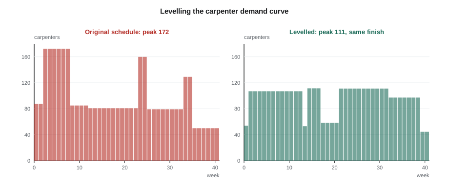
The histogram shows sharp peaks: about 172 carpenters in weeks 3 to 8, when the podium walls and decks overlap at full crew sizes, about 160 in weeks 24 and 25, when the upper tower floors start while the lower floors finish, and a smaller rise when the stairs and penthouse begin. Between the peaks, demand falls to about 80. A curve like this is expensive to staff: workers hired for the first peak must either be laid off in the dip, and may not come back, or kept on with too little to do. Luis's next step was to smooth it.
Levelling the curve
Resource levelling means adjusting the timing of activities within their float, or changing crew sizes and sequences, so that the workforce rises and falls more smoothly. On Elmwood, Luis stretched the podium walls and decks over longer durations with smaller crews working in parallel, started the lower tower floors two weeks later and the upper floors two weeks earlier, again with smaller crews working longer, and kept the stairs and penthouse finishing in week 41 as before. The total hours did not change and the finish date did not move, but the peak dropped from about 172 carpenters to about 111, roughly a third lower. A smaller, steadier crew is easier to recruit, easier to supervise and more productive, because workers learn the building and the repeated floor cycle.
Levelling has limits. Some activities have no float, some sequences are fixed by structure or by the owner's phasing, and some peaks cannot be avoided. In those cases, the plan should show when extra workers are needed early enough to request them from the hall or recruit them, and when they will be released, so that workers know what to expect.
Planning each trade and each subcontractor
The general contractor's workforce plan must cover the subcontractors as well, because on a building like Elmwood they supply most of the workers. At the start of the project, Calder Ridge asks each major subcontractor for its own labour curve, based on the master schedule, and combines them into a site-wide plan. The combined plan shows the peak number of workers on site, which drives decisions about site facilities, parking, hoisting, washrooms, lunchrooms and orientation capacity, as well as the risk that one trade's shortage will hold up others.
| Planning question | Why it matters on Elmwood |
|---|---|
| Peak workers on site by month | Sizing washrooms, lunchrooms, parking and hoist capacity for over 600 workers |
| Trades with the tightest labour market | Electricians and pipefitters were scarce; their curves were checked against the subcontractors' commitments on other projects |
| Overlaps between trades on the same floor | Too many crews on one floor reduces productivity and raises safety risk |
| Orientation load | Weeks with 40 or more new starts needed an extra orientation session |
| Apprentice and community targets | Planned hours by group, by trade, against the targets in lesson 6 |
What drives labour productivity
Labour productivity, the amount of work produced per worker-hour, varies enormously in construction, and much of the variation is under management's control. Studies of construction work consistently find that a large share of a typical worker's day is spent not on direct installation but on waiting for materials, information, equipment or other trades, travelling around the site, and reworking mistakes. Contractors that reduce these losses gain more than any wage difference.
| Factor | Effect on productivity | What supervisors can do |
|---|---|---|
| Material and information availability | Waiting is one of the largest losses | Look-ahead planning, constraint removal, kitting materials to the work face |
| Trade stacking and congestion | Too many crews in one area slow everyone | Plan the sequence and limit crews per floor |
| Extended overtime | Productivity falls after several weeks of long hours | Use overtime for specific short needs |
| Crew size and composition | Too small or too large a crew wastes time | Match crew size to the work; balance apprentices and journeypersons |
| Rework | Mistakes double the labour for that work | Clear drawings, first-installation reviews, quality checks |
| Weather and site conditions | Cold, heat, wind and mud reduce output | Protection, heating, scheduling sensitive work |
| Morale and supervision | Disorganized or disrespectful supervision lowers effort and raises turnover | Plan well, communicate, recognize good work |
| Learning curve | Repetitive work speeds up as crews learn it | Keep crews together through repeated cycles |
The real cost of overtime
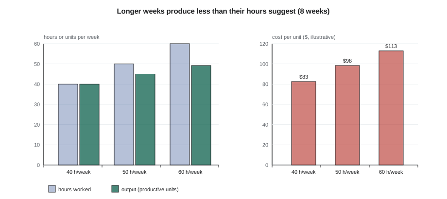
When a project falls behind, overtime is the quickest response, and for a week or two it works. Over longer periods, studies by industry groups and researchers have found that productivity per hour falls as long weeks continue: workers tire, mistakes increase, absenteeism rises, and the extra hours produce less than expected. Estimates vary, but a crew working 50 to 60 hours a week for more than a few weeks commonly loses 10 to 20 percent or more of its hourly productivity, and the loss grows the longer the schedule continues. Combined with premium pay, the cost per unit of work can rise sharply.
# Cost per unit of work for a carpenter crew under different weekly schedules over 8 weeks (illustrative)
base_rate = 82.54          # loaded cost of a straight-time hour ($)
ot_rate = 82.54 + 0.5 * 48.50 * 1.24   # loaded cost of a time-and-a-half hour ($)
schedules = {
    # name: (straight hours, overtime hours per week, productivity factor over 8 weeks)
    "40 h/week": (40, 0, 1.00),
    "50 h/week": (40, 10, 0.90),
    "60 h/week": (40, 20, 0.82),
}
for name, (st, ot, prod) in schedules.items():
    cost = st * base_rate + ot * ot_rate
    output = (st + ot) * prod          # units of work, where 1 unit = 1 productive straight-time hour
print(f"{name:10s} cost/week ${cost:8,.0f} output {output:5.1f} units cost per unit ${cost / output:6.2f} output vs 40 h: {output / 40:4.2f}x")40 h/week cost/week $ 3,302 output 40.0 units cost per unit $ 82.54 output vs 40 h: 1.00x 50 h/week cost/week $ 4,428 output 45.0 units cost per unit $ 98.39 output vs 40 h: 1.12x 60 h/week cost/week $ 5,554 output 49.2 units cost per unit $112.88 output vs 40 h: 1.23x
Working 60 hours a week for eight weeks produces only about 23 percent more output than working 40, at roughly 35 to 37 percent more cost per unit of work. If Luis needs 23 percent more output, a second, smaller crew or a second shift will often deliver it more cheaply, provided the workers and supervision are available. Overtime remains the right tool for short bursts: a pour that cannot stop, a week of recovery after a weather delay, or work that must be done when the hospital's existing building is quiet.
Measuring productivity on site
Calder Ridge measures productivity by comparing earned hours with actual hours. Each cost code has a budget of hours per unit of work. Each week the foreman reports quantities installed, which are converted to earned hours at the budget rate, and the payroll gives actual hours. A productivity factor below 1.0 means the crew is using more hours than planned.
# Weekly productivity by cost code: earned hours vs actual hours (Elmwood, week 22, illustrative)
codes = {
    # code: (budget hours per unit, units installed this week, actual hours)
    "column forms (each)":         (14.0, 18, 280),
    "deck forming (m2)":           (0.85, 980, 900),
    "wall forms (m2)":             (1.20, 240, 330),
    "stair forms (flight)":        (32.0, 3, 112),
}
te = ta = 0
for code, (rate, qty, actual) in codes.items():
    earned = rate * qty
    te += earned; ta += actual
    pf = earned / actual
    flag = "  <- review" if pf < 0.9 else ""
    print(f"{code:28s} earned {earned:6.0f} h  actual {actual:4d} h  PF {pf:4.2f}{flag}")
print(f"overall PF {te / ta:.2f}")column forms (each) earned 252 h actual 280 h PF 0.90 deck forming (m2) earned 833 h actual 900 h PF 0.93 wall forms (m2) earned 288 h actual 330 h PF 0.87 <- review stair forms (flight) earned 96 h actual 112 h PF 0.86 <- review overall PF 0.91
Wall forms and stair forms are running behind. When Luis asked the foremen why, the answers were specific: the wall forms were waiting for embedded conduit from the electrical subcontractor, and the stair crew had been short a journeyperson for two days. Neither was a question of effort. The productivity numbers are useful only as a way of finding and removing obstacles, and Calder Ridge's supervisors are taught to ask what got in the crew's way before asking whether the crew worked hard enough.
Planning the end of the job
Workforce plans often stop at the peak, but the run-down matters too. As each trade finishes, workers must be released in an orderly way that respects the collective agreement's layoff provisions and the employment standards notice rules, keeps the most versatile workers for the punch list, and gives good workers a path to the next project. Calder Ridge holds a monthly meeting during the last six months of each project to match workers finishing on one job with needs on the next, which has done more for retention than any bonus.
Common mistakes
MistakeStaffing to a raw schedule with sharp peaks and dips.
InsteadLevel the labour curve within float and plan hiring and releases around unavoidable peaks.
MistakePlanning only the general contractor's own crews.
InsteadCombine subcontractors' labour curves into a site-wide plan that drives facilities and risk decisions.
MistakeUsing sustained overtime to recover a long delay.
InsteadRecognize that productivity falls over long weeks; consider added crews or shifts for sustained recovery.
MistakeReading a low productivity factor as a lack of effort.
InsteadAsk what obstacles the crew faced and remove them.
MistakeEnding the workforce plan at the peak.
InsteadPlan the run-down and carry good workers to the next project.
Summary and key terms
- Labour is scarce: over 1.4 million new trades workers are needed by 2033, and retirements are high.
- Activity hours spread over durations give a labour histogram and an S-curve.
- Levelling smooths the curve, lowers the peak and keeps crews steadier and more productive.
- The site-wide plan must include subcontractors and drive facilities, hoisting and orientation capacity.
- Waiting, congestion, overtime, rework, weather and supervision drive productivity.
- Sustained overtime raises cost per unit of work because productivity falls as long weeks continue.
- Earned versus actual hours show where to look; the response is removing obstacles.
- Plan the run-down and the transfer of workers to the next project.
- Labour histogram
- A chart of workers needed by trade in each period of the project.
- S-curve
- The cumulative curve of labour hours or cost over a project.
- Resource levelling
- Adjusting activity timing or crews to smooth workforce demand.
- Trade stacking
- Several trades working in the same area at once, often reducing productivity.
- Earned hours
- Budgeted hours for the quantity of work actually installed.
- Productivity factor
- Earned hours divided by actual hours; below 1.0 means more hours than planned.
- Run-down
- The orderly reduction of the workforce as a project finishes.
Practice problems
Work each problem on paper first, then reveal the answer to check.
What was the peak carpenter demand in the raw Elmwood schedule, and when?
Show answer
About 172 carpenters, from week 3, when the podium walls and decks overlapped.
Why is a smoother labour curve more productive?
Show answer
A steadier crew is easier to recruit and supervise and learns the building and repeated cycles.
In the overtime example, how much more output did 60-hour weeks produce than 40-hour weeks, and at what change in cost per unit?
Show answer
About 23 percent more output at roughly 35 to 37 percent more cost per unit.
Which two cost codes were flagged in week 22, and what were the causes?
Show answer
Wall forms, waiting for electrical embeds, and stair forms, short a journeyperson.
What did Calder Ridge's monthly run-down meetings achieve?
Show answer
They matched workers finishing on one job with needs on the next, improving retention.
Lesson quiz · 5 questions
Score 60% or more to complete this lesson.
Create a free account to save your progress, take quizzes and earn a certificate.