Probabilistic reasoning and Bayesian networks

Logic lets an agent conclude what must be true, but real agents rarely have that luxury. A commuter who is late might have been in a crash, or stuck behind a power outage at the traffic lights, or delayed by a snowstorm that caused both; a doctor sees symptoms compatible with several diseases; a robot's sensor readings are noisy. In such cases the rational thing is to reason with degrees of belief and to act on the best bet. Probability theory provides the language. Bayesian networks provide the structure that makes probabilistic reasoning compact and efficient, and they were among the ideas that ended the second AI winter.

This lesson reviews the probability needed, introduces Bayesian networks and their semantics, shows how to read independence from a network with d-separation, and develops exact inference by enumeration and variable elimination and approximate inference by rejection sampling and likelihood weighting. AI-320 continues with learning network parameters and structure, Markov chain Monte Carlo, dynamic networks over time and causal inference, and ROB-310 applies Bayes filters to robot localization.

Why probability?

Trying to cope with uncertainty in logic quickly fails. A rule such as Late ⇒ Crash is simply false, since there are many other causes of lateness; Late ⇒ Crash ∨ Outage ∨ Storm ∨ … never ends; and the causal direction Crash ⇒ Late is not always true either. Logic fails here for three reasons: laziness (listing every exception is too much work), theoretical ignorance (we do not know the complete theory of the domain) and practical ignorance (even with complete rules, we cannot observe everything relevant). Probability summarizes the uncertainty that comes from all three. A rational agent assigns degrees of belief, updates them with evidence by the rules of probability, and in lesson 10 chooses the action with the highest expected utility.

Probability is the right calculus for degrees of belief, not just one choice among many: de Finetti showed that an agent whose beliefs violate the axioms of probability can be offered a set of bets, each acceptable by its own lights, that guarantees it loses money whatever happens. Any coherent system of degrees of belief must therefore obey the axioms.

A quick review

A random variable has a domain of possible values; here all variables are Boolean, and we write s for S = true and ¬s for S = false. A probability distribution P(X) gives the probability of each value. The joint distribution P(X1, …, Xn) gives the probability of every combination of values, and from it any question can be answered by summing (marginalization) and dividing (conditioning). The conditional probability of a given b is P(a | b) = P(a ∧ b) / P(b). Rearranging gives the product rule, P(a ∧ b) = P(a | b) P(b), and from it Bayes' rule:

Bayes' rule is how an agent reasons from observed effects back to hidden causes using the causal knowledge it actually has: how likely the effect is given each cause. Two variables X and Y are independent if P(X, Y) = P(X) P(Y), and conditionally independent given Z if P(X, Y | Z) = P(X | Z) P(Y | Z). Independence is what makes large problems tractable. The full joint distribution of n Boolean variables needs 2^n − 1 numbers; with 30 variables, that is more than a billion. Conditional independence lets us factor it into small pieces.

Bayesian networks

A Bayesian network is a directed acyclic graph in which each node is a random variable and each node X has a conditional probability table (CPT) giving P(X | Parents(X)) for every combination of its parents' values. Informally, an arrow from X to Y means that X has a direct influence on Y, and typically that X is a cause of Y. Judea Pearl developed Bayesian networks in the 1980s, and in 2011 he received the Turing Award for this work and for his later work on causal reasoning.

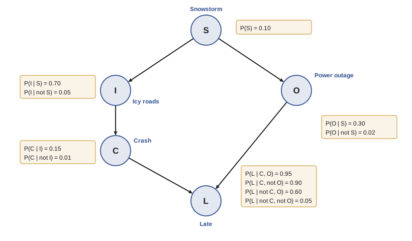
The network's semantics is that the full joint distribution is the product of the local conditional distributions:

For the commute network, P(s, i, o, c, l) = P(s) P(i | s) P(o | s) P(c | i) P(l | c, o). This holds because each node is conditionally independent of its other predecessors, in an ordering consistent with the graph, given its parents. The saving is large: our five Boolean variables need 11 numbers in their CPTs instead of 31 for the full joint, and in general a network in which each of n Boolean variables has at most k parents needs at most n·2^k numbers rather than 2^n − 1. A medical network with 400 variables and at most five parents each needs at most 12,800 numbers, against 2^400 for the full joint.

Building a network is easiest in the causal direction: add root causes first, then the variables they directly influence, choosing as parents of each new node a minimal set of existing nodes that directly influence it. Building in the diagnostic direction (symptoms first, then causes) gives networks with more arcs and CPT entries that are harder to estimate, because experts think more naturally about P(symptom | disease) than P(disease | symptom). In practice CPTs come from experts, from data, or from both; AI-320 covers learning them.

Exact inference by enumeration

The basic task is to compute the posterior distribution P(X | e) of a query variable X given observed evidence e, summing over the remaining hidden variables y:

where α is a normalizing constant that makes the distribution sum to 1. Each term P(X, e, y) is a product of CPT entries, by the network semantics. The program computes queries by summing the full joint in exactly this way.

# A Bayesian network for a winter morning commute. Each node lists its parents and
# P(node = True | parent values). S: snowstorm, I: icy roads, O: power outage, C: crash, L: late.
NET = {
    "S": ((), {(): 0.10}),
    "I": (("S",), {(True,): 0.70, (False,): 0.05}),
    "O": (("S",), {(True,): 0.30, (False,): 0.02}),
    "C": (("I",), {(True,): 0.15, (False,): 0.01}),
    "L": (("C", "O"), {(True, True): 0.95, (True, False): 0.90, (False, True): 0.60, (False, False): 0.05}),
}
ORDER = ["S", "I", "O", "C", "L"]                     # a topological order: parents before children

def p(var, value, world):
    parents, cpt = NET[var]
    pt = cpt[tuple(world[q] for q in parents)]
    return pt if value else 1 - pt

from itertools import product

def joint(world):                                       # the chain rule for Bayesian networks
    prob = 1.0
    for v in ORDER: prob *= p(v, world[v], world)
    return prob

def query(var, evidence):
    """P(var = True | evidence) by summing the full joint over the hidden variables."""
    totals = {True: 0.0, False: 0.0}
    hidden = [v for v in ORDER if v != var and v not in evidence]
    for value in (True, False):
        for vals in product((True, False), repeat=len(hidden)):
            world = {**evidence, var: value, **dict(zip(hidden, vals))}
            totals[value] += joint(world)
    return totals[True] / (totals[True] + totals[False])

params = sum(len(cpt) for _, cpt in NET.values())
print(f"network parameters: {params}; full joint table over 5 Boolean variables: {2 ** 5 - 1}")
print(f"sum of the joint over all 32 worlds: {sum(joint(dict(zip(ORDER, v))) for v in product((True, False), repeat=5)):.6f}")
for var, ev in [("S", {}), ("L", {}), ("S", {"L": True}), ("C", {"L": True}),
                ("S", {"L": True, "C": False}), ("O", {"L": True}), ("O", {"L": True, "C": True})]:
    given = ", ".join(f"{k}={'T' if v else 'F'}" for k, v in ev.items()) or "nothing"
    print(f"P({var}=T | {given:9}) = {query(var, ev):.4f}")

network parameters: 11; full joint table over 5 Boolean variables: 31
sum of the joint over all 32 worlds: 1.000000
P(S=T | nothing  ) = 0.1000
P(L=T | nothing  ) = 0.0968
P(S=T | L=T      ) = 0.3002
P(C=T | L=T      ) = 0.2445
P(S=T | L=T, C=F ) = 0.2622
P(O=T | L=T      ) = 0.3103
P(O=T | L=T, C=T ) = 0.1423

Several patterns of reasoning appear. Diagnostic reasoning goes from effect to cause: learning that the commuter is late raises the probability of a snowstorm from 0.10 to 0.30. Causal reasoning goes the other way: the prior probability of being late is about 0.097, and it would rise if we observed a storm. The most interesting pattern is intercausal reasoning, or explaining away. Lateness raises the probability of a power outage to 0.31; but if we also learn there was a crash, the probability of an outage falls to 0.14, because the crash already explains the lateness. The two causes C and O are independent a priori except through the storm, yet observing their common effect makes them compete. Explaining away is a pattern that rule-based systems found very hard to capture and Bayesian networks get for free.

Conditional independence and d-separation

The network structure tells us which independence statements hold, whatever the numbers in the CPTs. Two basic facts follow from the semantics: each node is conditionally independent of its non-descendants given its parents, and each node is conditionally independent of all other nodes given its Markov blanket (its parents, its children and its children's other parents). The general criterion, d-separation, decides whether sets of variables X and Y are conditionally independent given evidence Z by examining every undirected path between them.

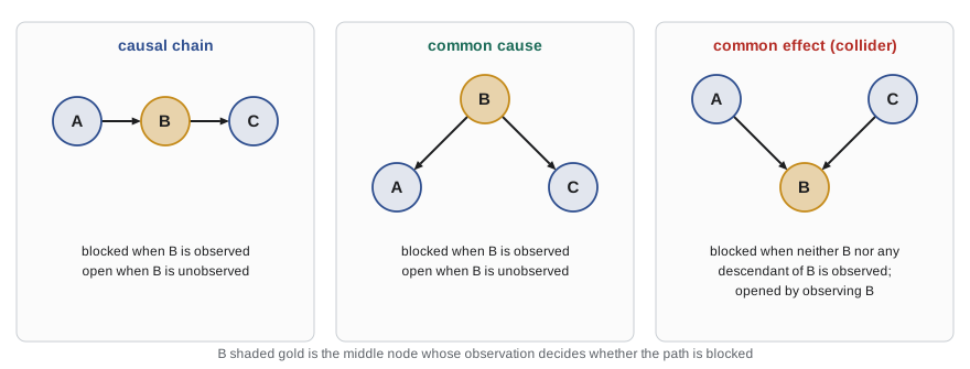
A path is blocked by Z if it contains a node B where one of three things happens: B is the middle of a chain (A → B → C) and B is in Z; B is a common cause (A ← B → C) and B is in Z; or B is a common effect, a collider (A → B ← C), and neither B nor any of its descendants is in Z. X and Y are d-separated by Z, and therefore conditionally independent given Z in every distribution the network can represent, if every path between them is blocked. The collider rule is the formal version of explaining away: two causes become dependent when their common effect is observed.

# A Bayesian network for a winter morning commute. Each node lists its parents and
# P(node = True | parent values). S: snowstorm, I: icy roads, O: power outage, C: crash, L: late.
NET = {
    "S": ((), {(): 0.10}),
    "I": (("S",), {(True,): 0.70, (False,): 0.05}),
    "O": (("S",), {(True,): 0.30, (False,): 0.02}),
    "C": (("I",), {(True,): 0.15, (False,): 0.01}),
    "L": (("C", "O"), {(True, True): 0.95, (True, False): 0.90, (False, True): 0.60, (False, False): 0.05}),
}
ORDER = ["S", "I", "O", "C", "L"]                     # a topological order: parents before children

def p(var, value, world):
    parents, cpt = NET[var]
    pt = cpt[tuple(world[q] for q in parents)]
    return pt if value else 1 - pt

# d-separation: can information flow from X to Y given the evidence set Z? (the reachable algorithm)
CHILDREN = {v: [c for c in ORDER if v in NET[c][0]] for v in ORDER}

def d_separated(x, y, z):
    # ancestors of the evidence (a collider is active if it or a descendant is observed)
    anc, stack = set(), list(z)
    while stack:
        v = stack.pop()
        if v not in anc: anc.add(v); stack.extend(NET[v][0])
    visited, stack = set(), [(x, "up")]                 # "up": arrived from a child; "down": from a parent
    while stack:
        v, d = stack.pop()
        if (v, d) in visited: continue
        visited.add((v, d))
        if v == y: return False                          # an active trail reaches y
        if d == "up" and v not in z:
            stack += [(q, "up") for q in NET[v][0]] + [(c, "down") for c in CHILDREN[v]]
        elif d == "down":
            if v not in z: stack += [(c, "down") for c in CHILDREN[v]]   # chain through v
            if v in anc:   stack += [(q, "up") for q in NET[v][0]]       # collider opened by evidence
    return True

for x, y, z in [("I", "O", []), ("I", "O", ["S"]), ("S", "L", []), ("S", "L", ["C", "O"]),
                ("C", "O", []), ("C", "O", ["L"]), ("I", "L", ["C"]), ("I", "L", ["C", "S"])]:
    verdict = "independent" if d_separated(x, y, set(z)) else "may be dependent"
    print(f"{x} and {y} given {{{', '.join(z)}}}: {verdict}")

I and O given {}: may be dependent
I and O given {S}: independent
S and L given {}: may be dependent
S and L given {C, O}: independent
C and O given {}: may be dependent
C and O given {L}: may be dependent
I and L given {C}: may be dependent
I and L given {C, S}: independent

Each answer can be checked against the graph. Icy roads and outages are dependent through their common cause, the storm, but independent once the storm is known. Crash and outage are dependent a priori through the storm, and remain dependent given lateness because L is a collider on the path C → L ← O. Knowing whether there was a crash does not make icy roads irrelevant to lateness, because another path runs from I up to S and down through O to L; observing S as well blocks that path.

Variable elimination

Enumeration recomputes the same products many times. In P(l) = Σs Σi Σo Σc P(s) P(i | s) P(o | s) P(c | i) P(l | c, o), the term P(c | i) does not depend on o, and P(i | s) does not depend on c or o. Moving each factor outside the sums that do not involve it, and storing intermediate results as small tables called factors, avoids the repetition. This is variable elimination: sum out one hidden variable at a time, multiplying together only the factors that mention it.

# A Bayesian network for a winter morning commute. Each node lists its parents and
# P(node = True | parent values). S: snowstorm, I: icy roads, O: power outage, C: crash, L: late.
NET = {
    "S": ((), {(): 0.10}),
    "I": (("S",), {(True,): 0.70, (False,): 0.05}),
    "O": (("S",), {(True,): 0.30, (False,): 0.02}),
    "C": (("I",), {(True,): 0.15, (False,): 0.01}),
    "L": (("C", "O"), {(True, True): 0.95, (True, False): 0.90, (False, True): 0.60, (False, False): 0.05}),
}
ORDER = ["S", "I", "O", "C", "L"]                     # a topological order: parents before children

def p(var, value, world):
    parents, cpt = NET[var]
    pt = cpt[tuple(world[q] for q in parents)]
    return pt if value else 1 - pt

# Computing P(L = True) two ways: summing the full joint, and pushing sums inward (variable elimination).
from itertools import product
mults = 0
def times(*xs):
    global mults
    out = 1.0
    for x in xs[1:]: mults += 1
    for x in xs: out *= x
    return out

# 1. enumeration: one product of five factors for each of the 16 worlds with L = True
total = sum(times(*(p(v, w[v], w) for v in ORDER))
            for vals in product((True, False), repeat=4)
            for w in [dict(zip(["S", "I", "O", "C"], vals), L=True)])
print(f"enumeration:          P(L=T) = {total:.6f} using {mults} multiplications")

# 2. variable elimination in the order I, S, C, O. Each factor is a small table.
mults = 0
B = (True, False)
f_C_given_S = {(c, s): sum(times(p("I", i, {"S": s}), p("C", c, {"I": i})) for i in B) for c in B for s in B}  # sum out I
f_C_O = {(c, o): sum(times(p("S", s, {}), p("O", o, {"S": s}), f_C_given_S[(c, s)]) for s in B)
         for c in B for o in B}                                                                           # sum out S
f_O = {o: sum(times(f_C_O[(c, o)], p("L", True, {"C": c, "O": o})) for c in B) for o in B}                # sum out C
ve = sum(f_O.values())                                                                                    # sum out O
print(f"variable elimination: P(L=T) = {ve:.6f} using {mults} multiplications")

enumeration:          P(L=T) = 0.096812 using 64 multiplications
variable elimination: P(L=T) = 0.096812 using 28 multiplications

Even in a five-node network the saving is more than half; in large networks it is the difference between feasible and impossible. The cost of variable elimination depends on the order in which variables are eliminated, because that determines the size of the largest intermediate factor. For polytrees, networks with at most one undirected path between any two nodes, exact inference takes time linear in the size of the network. In general, exact inference is NP-hard (it can encode 3-SAT), and its cost grows exponentially with the treewidth of the network, the same structural measure that governed CSPs in lesson 6. Clustering (junction tree) algorithms, used in commercial tools, build on the same idea.

Approximate inference by sampling

When exact inference is too expensive, we can estimate probabilities by generating random samples. Direct (prior) sampling draws each variable in topological order from its CPT given its already-sampled parents; the fraction of samples with a property estimates its probability, and the estimate converges to the truth as the number of samples grows (it is consistent). To answer conditional queries, rejection sampling throws away every sample that disagrees with the evidence and counts among the rest. Its problem is waste: if the evidence has probability 0.001, it discards 999 samples in 1,000.

Likelihood weighting avoids rejection. It fixes the evidence variables to their observed values and samples only the others, and it weights each sample by the likelihood of the evidence given the sampled values, the product of P(e_i | parents(E_i)) over the evidence variables. The weighted fraction of samples with X = true estimates P(x | e), and the estimate is consistent. Its weakness is that evidence affects only the sampling of variables downstream of it; when evidence is at the leaves and is unlikely, most samples get tiny weights and a few dominate.

# A Bayesian network for a winter morning commute. Each node lists its parents and
# P(node = True | parent values). S: snowstorm, I: icy roads, O: power outage, C: crash, L: late.
NET = {
    "S": ((), {(): 0.10}),
    "I": (("S",), {(True,): 0.70, (False,): 0.05}),
    "O": (("S",), {(True,): 0.30, (False,): 0.02}),
    "C": (("I",), {(True,): 0.15, (False,): 0.01}),
    "L": (("C", "O"), {(True, True): 0.95, (True, False): 0.90, (False, True): 0.60, (False, False): 0.05}),
}
ORDER = ["S", "I", "O", "C", "L"]                     # a topological order: parents before children

def p(var, value, world):
    parents, cpt = NET[var]
    pt = cpt[tuple(world[q] for q in parents)]
    return pt if value else 1 - pt

import random
from itertools import product

def exact(var, evidence):
    tot = {True: 0.0, False: 0.0}
    for vals in product((True, False), repeat=5):
        w = dict(zip(ORDER, vals))
        if all(w[k] == v for k, v in evidence.items()):
            pr = 1.0
            for v in ORDER: pr *= p(v, w[v], w)
            tot[w[var]] += pr
    return tot[True] / (tot[True] + tot[False])

def prior_sample(rng):
    world = {}
    for v in ORDER: world[v] = rng.random() < p(v, True, world)
    return world

def rejection(var, evidence, n, rng):
    kept = hits = 0
    for _ in range(n):
        w = prior_sample(rng)
        if all(w[k] == v for k, v in evidence.items()):
            kept += 1; hits += w[var]
    return (hits / kept if kept else float("nan")), kept

def likelihood_weighting(var, evidence, n, rng):
    num = den = 0.0
    for _ in range(n):
        world, weight = {}, 1.0
        for v in ORDER:
            if v in evidence:
                world[v] = evidence[v]; weight *= p(v, evidence[v], world)   # fix evidence, weight it
            else:
                world[v] = rng.random() < p(v, True, world)
        num += weight * world[var]; den += weight
    return num / den

rng = random.Random(366)
for evidence in ({"L": True}, {"C": True, "O": True}):
    truth = exact("S", evidence)
    ev = ", ".join(f"{k}=T" for k in evidence)
    print(f"P(S=T | {ev}) exact {truth:.4f}")
    for n in (100, 1000, 10000):
        r, kept = rejection("S", evidence, n, rng)
        lw = likelihood_weighting("S", evidence, n, rng)
        shown = f"{r:.4f}" if kept else "undefined"
        print(f"  n={n:6}: rejection {shown:>9} (kept {kept:5} samples)   likelihood weighting {lw:.4f}")

P(S=T | L=T) exact 0.3002
  n=   100: rejection    0.3000 (kept    20 samples)   likelihood weighting 0.2732
  n=  1000: rejection    0.2584 (kept    89 samples)   likelihood weighting 0.2849
  n= 10000: rejection    0.2782 (kept   985 samples)   likelihood weighting 0.3074
P(S=T | C=T, O=T) exact 0.9137
  n=   100: rejection undefined (kept     0 samples)   likelihood weighting 0.9546
  n=  1000: rejection    0.7500 (kept     4 samples)   likelihood weighting 0.9111
  n= 10000: rejection    0.8333 (kept    36 samples)   likelihood weighting 0.9101

With common evidence (lateness, probability about 0.1), both methods approach the exact answer of 0.30 as samples increase, though rejection sampling uses only about one sample in ten. With rare evidence (a crash and an outage together), rejection sampling keeps no samples at all out of 100 and only 36 out of 10,000, so its estimates are useless, while likelihood weighting is close to the exact 0.91 after 1,000 samples. Markov chain Monte Carlo methods such as Gibbs sampling go further: they wander through the space of complete assignments, resampling one variable at a time given its Markov blanket, and they handle evidence anywhere in the network. AI-320 develops them.

Worked examples