Adversarial search and games

So far the agent has been alone: the world changed only when the agent acted. In a game, another agent acts too, and it wants the opposite outcome. A plan such as 'go here, then there' is useless when the opponent's replies decide where you end up. The agent needs a strategy, a choice of move for every position the opponent might lead it into. This lesson covers the classical theory of two-player, zero-sum games of perfect information: minimax, alpha–beta pruning, evaluation functions and depth-limited search. It then handles chance with expectimax, introduces Monte Carlo tree search, and tells the story of game-playing programs from checkers to Go, a story in which the University of Alberta plays a central part.

Games have been a proving ground for AI since Turing and Shannon wrote chess programs on paper around 1950. They are attractive because the rules are precise, success is measurable and the state spaces are enormous. Chess has roughly 10^44 legal positions and Go about 10^170, far beyond any exhaustive search. Game theory in the economist's sense, including mixed strategies and equilibria for simultaneous-move games, is treated in AI-470 and AI-330; here we stay with turn-taking search.

Games as search problems

A two-player game is defined by an initial state, a function PLAYER(s) saying whose turn it is, actions, a transition model, a terminal test, and a utility function UTILITY(s, p) giving the final payoff to player p at a terminal state. In a zero-sum game the players' payoffs always sum to a constant (+1 and −1, or 1/2 and 1/2 for a draw), so one player's gain is the other's loss. We call the players MAX, who moves first and wants high utility, and MIN, who wants low utility. The initial state, actions and transition model define a game tree whose levels alternate between MAX and MIN.

Minimax

The minimax value of a state is the utility, for MAX, of reaching a terminal state if both players play optimally from there on. It is defined recursively:

MAX chooses the move leading to the state with the highest minimax value. This is optimal against an optimal opponent, and against a weaker opponent it can only do better, though another strategy might exploit a weak opponent more. The minimax algorithm computes these values by a complete depth-first exploration of the game tree, so its time is O(b^m) and its space O(bm) for maximum depth m. Tic-tac-toe is small enough to search completely, as the program shows: from the empty board, minimax visits 549,946 nodes and confirms the folk result that perfect play is a draw.

# Tic-tac-toe solved by minimax, then by alpha-beta: count the nodes each visits.
LINES = [(0, 1, 2), (3, 4, 5), (6, 7, 8), (0, 3, 6), (1, 4, 7), (2, 5, 8), (0, 4, 8), (2, 4, 6)]
def winner(b):
    for i, j, k in LINES:
        if b[i] != "." and b[i] == b[j] == b[k]: return b[i]
    return None
def moves(b): return [i for i in range(9) if b[i] == "."]
def play(b, i, p): return b[:i] + p + b[i + 1:]

count = 0
def minimax(b, player):
    """Value of board b for X (+1 win, 0 draw, -1 loss) with `player` to move."""
    global count; count += 1
    w = winner(b)
    if w: return 1 if w == "X" else -1
    if "." not in b: return 0
    vals = [minimax(play(b, i, player), "O" if player == "X" else "X") for i in moves(b)]
    return max(vals) if player == "X" else min(vals)

def alphabeta(b, player, alpha=-2, beta=2, order=None):
    global count; count += 1
    w = winner(b)
    if w: return 1 if w == "X" else -1
    if "." not in b: return 0
    ms = moves(b) if order is None else sorted(moves(b), key=order)
    if player == "X":
        v = -2
        for i in ms:
            v = max(v, alphabeta(play(b, i, "X"), "O", alpha, beta, order))
            alpha = max(alpha, v)
            if alpha >= beta: break                 # beta cut-off: O will never allow this
        return v
    v = 2
    for i in ms:
        v = min(v, alphabeta(play(b, i, "O"), "X", alpha, beta, order))
        beta = min(beta, v)
        if alpha >= beta: break                     # alpha cut-off: X will never allow this
    return v

empty = "." * 9
v = minimax(empty, "X"); print(f"minimax:              value {v:+d}, nodes visited {count:,}")
count = 0; v = alphabeta(empty, "X"); print(f"alpha-beta:           value {v:+d}, nodes visited {count:,}")
middle_first = lambda i: [4, 0, 2, 6, 8, 1, 3, 5, 7].index(i)    # try the middle, then corners
count = 0; v = alphabeta(empty, "X", order=middle_first); print(f"alpha-beta, ordered:  value {v:+d}, nodes visited {count:,}")

seen = set()
def distinct(b, player):
    if b in seen: return
    seen.add(b)
    if winner(b) or "." not in b: return
    for i in moves(b): distinct(play(b, i, player), "O" if player == "X" else "X")
distinct(empty, "X")
print(f"distinct positions reachable: {len(seen):,} (a transposition table visits each once)")

minimax:              value +0, nodes visited 549,946
alpha-beta:           value +0, nodes visited 18,297
alpha-beta, ordered:  value +0, nodes visited 7,275
distinct positions reachable: 5,478 (a transposition table visits each once)

Alpha–beta pruning

Minimax looks at every node, but many of them cannot affect the decision. Suppose MAX has already found a move worth 3, and while examining a second move discovers that MIN can reply with something worth 2 for MAX. There is no need to look at MIN's other replies: the second move is worth at most 2, so MAX will not choose it. Alpha–beta pruning formalizes this. It passes two bounds down the tree: α, the best value MAX can already guarantee along the current path, and β, the best (lowest) value MIN can guarantee. Whenever α ≥ β at a node, the remaining children are pruned, because a rational player higher up will never let play reach this node.

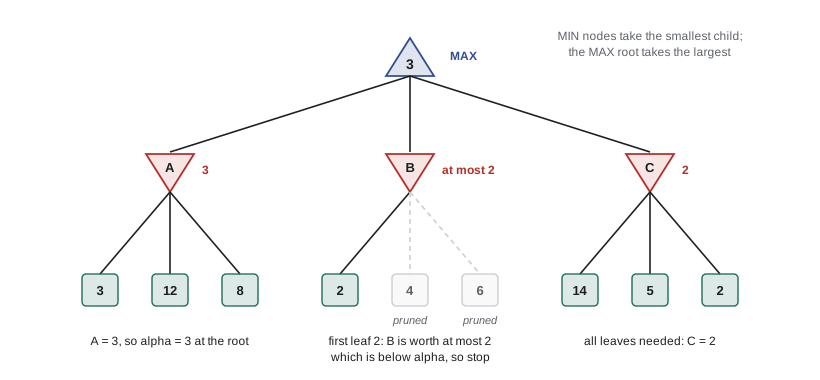
Alpha–beta returns exactly the minimax value; pruning only skips work. How much it skips depends on move order. If the best move at every node is examined first, alpha–beta examines about O(b^(m/2)) nodes instead of O(b^m), which means it can search twice as deep in the same time. With random ordering the figure is about O(b^(3m/4)). On tic-tac-toe, alpha–beta cuts 549,946 nodes to 18,297, and simply trying the centre and corners first cuts that to 7,275. Real programs order moves with cheap tricks: captures first, the best move found by a previous shallower search first (the principle behind iterative deepening in game search), and killer moves that caused cut-offs elsewhere at the same depth.

Another large saving comes from transpositions: different move orders that reach the same position. Tic-tac-toe has only 5,478 distinct positions reachable from the empty board, against hundreds of thousands of paths. A transposition table, a hash table of positions already evaluated, lets the search look up a position's value instead of recomputing it. Chess programs use transposition tables with billions of entries, indexed by Zobrist hashing, which updates a position's hash incrementally with an exclusive-or for each piece moved.

Evaluation functions and depth limits

For any interesting game, even alpha–beta cannot reach the terminal states. Claude Shannon proposed the solution in 1950: cut the search off at some depth and apply a heuristic evaluation function EVAL(s) that estimates the expected utility of the position. The search then backs up these estimates instead of true utilities. An evaluation function should order terminal states the same way as the true utility, be fast to compute, and correlate strongly with the actual chances of winning.

Most classical evaluation functions are weighted linear functions of features: EVAL(s) = w1·f1(s) + … + wn·fn(s). In chess the features include material (a pawn 1, knight and bishop 3, rook 5, queen 9), mobility, king safety and pawn structure; in checkers, the number of men and kings, control of the centre and back-row defence. The weights can be set by hand or learned. Arthur Samuel's checkers program at IBM, starting in the 1950s, was among the first programs to learn its own evaluation weights by playing against itself, which is where the term machine learning entered common use.

Cutting off search creates problems of its own. A position might look good just before the opponent captures a queen; the evaluation should be applied only to quiescent positions, so programs extend the search through captures and checks until things settle (quiescence search). The horizon effect is subtler: a program facing an unavoidable loss may make delaying moves that push the loss just beyond its search depth, sacrificing material for nothing. Singular extensions, which search deeper along a move that is clearly better than all alternatives, reduce it. Forward pruning, which ignores moves that look bad at a shallow depth, saves time at the risk of missing a deep resource.

Chance: expectimax

Many games include dice, shuffled cards or other random events. Backgammon is the classic example. Its game tree contains chance nodes, at which nature chooses an outcome with known probabilities. The value of a chance node is the expected value of its children, which gives expectiminimax: MAX nodes take the maximum, MIN nodes the minimum and chance nodes the probability-weighted average. When no adversary is present at all, only an agent and a random environment, the same idea is called expectimax, and it leads directly to the decision theory of lesson 10.

# Minimax versus expectimax when an opponent (or nature) is not adversarial.
# MAX chooses a lever; then a chance node picks an outcome with the given probabilities.
levers = {
    "safe":  [(1.0, 40)],
    "risky": [(0.5, 100), (0.5, 0)],
    "steady": [(0.9, 45), (0.1, 0)],
}
def minimax_value(outcomes): return min(v for _, v in outcomes)          # assume the worst
def expectimax_value(outcomes): return sum(p * v for p, v in outcomes)   # average over chance
for name, f in [("minimax", minimax_value), ("expectimax", expectimax_value)]:
    vals = {k: f(o) for k, o in levers.items()}
    best = max(vals, key=vals.get)
    print(f"{name:10} values {vals}  choose {best}")

# Expectimax depends on the scale of the evaluation, not just its order.
squash = lambda v: v ** 0.5                       # an order-preserving change of evaluation
vals = {k: round(sum(p * squash(v) for p, v in o), 2) for k, o in levers.items()}
print(f"expectimax after sqrt   values {vals}  choose {max(vals, key=vals.get)}")
vals = {k: min(squash(v) for _, v in o) for k, o in levers.items()}
print(f"minimax after sqrt      choose {max(vals, key=vals.get)} (unchanged)")

minimax    values {'safe': 40, 'risky': 0, 'steady': 0}  choose safe
expectimax values {'safe': 40.0, 'risky': 50.0, 'steady': 40.5}  choose risky
expectimax after sqrt   values {'safe': 6.32, 'risky': 5.0, 'steady': 6.04}  choose safe
minimax after sqrt      choose safe (unchanged)

The program makes two points. First, minimax assumes the worst, which is right against an opponent but overly pessimistic against dice: expectimax picks the risky lever with expected value 50, while minimax picks the safe 40. Second, minimax decisions are unchanged by any order-preserving transformation of the evaluation function, but expectimax decisions are not. Taking square roots of the payoffs, which preserves their order, switches expectimax's choice back to the safe lever. So for games of chance the evaluation function must be a positive linear transformation of the probability of winning, or more generally of expected utility; its actual numbers matter, not just its ranking. Lesson 10 makes this precise with utility theory.

Chance multiplies the branching factor. With 21 distinct dice rolls in backgammon and about 20 legal moves for each roll, a search four moves deep examines more than a billion positions. Gerald Tesauro's TD-Gammon (1992) therefore combined a shallow two- or three-ply search with an evaluation function learned by temporal-difference reinforcement learning in self-play, and reached the level of the world's best players. That combination, learned evaluation plus search, is the template for AlphaZero.

Monte Carlo tree search

For Go, both pieces of the classical approach failed. The branching factor is about 250, so alpha–beta reaches only a few moves deep, and nobody could write a good evaluation function, because the value of a Go position depends on subtle patterns that resist simple features. Monte Carlo tree search (MCTS) avoids the evaluation function. It estimates the value of a position by playing many complete games, called playouts or rollouts, from that position to the end with a fast, mostly random policy, and averaging the results. It grows a search tree asymmetrically, spending playouts on the most promising moves.

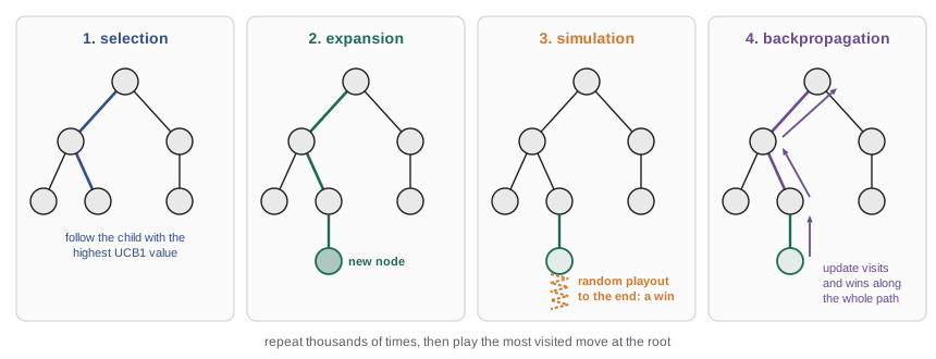
Each iteration has four steps. Selection walks down the tree from the root, at each node choosing a child by a selection policy. Expansion adds a new child to the tree when the walk reaches a node with untried moves. Simulation plays out a game from the new node using the playout policy. Backpropagation updates the win and visit counts of every node on the path with the result. After the time budget runs out, the program plays the move at the root that was visited most often. The selection policy must balance exploitation (moves that have won often) against exploration (moves tried rarely). The standard choice, UCT (upper confidence bounds applied to trees, Kocsis and Szepesvári, 2006), picks the child maximizing

where W(n) is the number of wins and N(n) the number of visits recorded for node n, and C is an exploration constant, often near √2. The first term favours moves with a high win rate; the second grows for moves that have been tried rarely relative to their parent. Csaba Szepesvári, one of UCT's inventors, is a professor at the University of Alberta. The program below implements UCT for tic-tac-toe and plays it, alternating first and second moves, against a random player and against a perfect minimax player.

# Monte Carlo tree search (UCT) for tic-tac-toe, played against a random player and a perfect player.
import math, random
from functools import lru_cache
LINES = [(0, 1, 2), (3, 4, 5), (6, 7, 8), (0, 3, 6), (1, 4, 7), (2, 5, 8), (0, 4, 8), (2, 4, 6)]
def winner(b):
    for i, j, k in LINES:
        if b[i] != "." and b[i] == b[j] == b[k]: return b[i]
    return "draw" if "." not in b else None
def moves(b): return [i for i in range(9) if b[i] == "."]
def play(b, i, p): return b[:i] + p + b[i + 1:]
other = {"X": "O", "O": "X"}

class Node:
    def __init__(self, board, player, parent=None, move=None):
        self.board, self.player, self.parent, self.move = board, player, parent, move
        self.children, self.untried = [], moves(board) if winner(board) is None else []
        self.n, self.w = 0, 0.0          # visits; wins for the player who moved INTO this node

def uct_search(board, player, iters, rng, c=1.4):
    root = Node(board, player)
    for _ in range(iters):
        node = root
        while not node.untried and node.children:                         # 1. selection
            node = max(node.children, key=lambda ch: ch.w / ch.n + c * math.sqrt(math.log(node.n) / ch.n))
        if node.untried:                                                   # 2. expansion
            m = node.untried.pop(rng.randrange(len(node.untried)))
            child = Node(play(node.board, m, node.player), other[node.player], node, m)
            node.children.append(child); node = child
        b, p = node.board, node.player                                     # 3. simulation
        while winner(b) is None:
            b = play(b, rng.choice(moves(b)), p); p = other[p]
        result = winner(b)
        while node is not None:                                            # 4. backpropagation
            node.n += 1
            mover = other[node.player]
            node.w += 1.0 if result == mover else (0.5 if result == "draw" else 0.0)
            node = node.parent
    return max(root.children, key=lambda ch: ch.n).move                    # most-visited move

@lru_cache(maxsize=None)
def value(b, p):                      # exact minimax value for X, used by the perfect player
    w = winner(b)
    if w: return {"X": 1, "O": -1, "draw": 0}[w]
    vals = [value(play(b, i, p), other[p]) for i in moves(b)]
    return max(vals) if p == "X" else min(vals)
def perfect(b, p, rng):
    best = max if p == "X" else min
    target = best(value(play(b, i, p), other[p]) for i in moves(b))
    return rng.choice([i for i in moves(b) if value(play(b, i, p), other[p]) == target])

def match(opponent, games, iters, seed):
    rng, tally = random.Random(seed), {"win": 0, "draw": 0, "loss": 0}
    for g in range(games):
        b, p = "." * 9, "X"
        mcts_plays = "X" if g % 2 == 0 else "O"
        while winner(b) is None:
            m = uct_search(b, p, iters, rng) if p == mcts_plays else opponent(b, p, rng)
            b = play(b, m, p); p = other[p]
        r = winner(b)
        tally["draw" if r == "draw" else ("win" if r == mcts_plays else "loss")] += 1
    return tally

random_player = lambda b, p, rng: rng.choice(moves(b))
for iters in (25, 200, 1000):
    print(f"UCT with {iters:4} playouts per move  vs random: {match(random_player, 20, iters, 1)}"
          f"   vs perfect: {match(perfect, 10, iters, 2)}")

UCT with   25 playouts per move  vs random: {'win': 15, 'draw': 2, 'loss': 3}   vs perfect: {'win': 0, 'draw': 4, 'loss': 6}
UCT with  200 playouts per move  vs random: {'win': 19, 'draw': 1, 'loss': 0}   vs perfect: {'win': 0, 'draw': 7, 'loss': 3}
UCT with 1000 playouts per move  vs random: {'win': 19, 'draw': 1, 'loss': 0}   vs perfect: {'win': 0, 'draw': 9, 'loss': 1}

With only 25 playouts per move, UCT already beats a random player most of the time but loses most games against perfect play. With 1,000 playouts it wins nearly every game against the random player and draws nine of ten against the perfect player, without knowing anything about tic-tac-toe except the rules. Its remaining loss shows the weakness of random playouts: a move that wins most random continuations can still lose to an opponent who finds the one refutation. MCTS is an anytime algorithm: it can be stopped whenever time runs out and return its current best move, which suits dynamic environments and real-time play.

Game-playing programs: a short history

Chinook deserves a closer look, because it shows the classical methods at their most powerful. Jonathan Schaeffer's team at the University of Alberta began the project in 1989. In 1994 Chinook played Marion Tinsley, the greatest checkers player in history, for the world title; Tinsley withdrew for health reasons after six drawn games, and Chinook went on to defend the title. The team then set out to solve the game. After 18 years of computation, in 2007 they published a proof in the journal Science that the standard game is a draw: Chinook can never lose, and a perfect opponent can never lose to it. With about 5 × 10^20 positions, checkers was the largest game solved at the time.

AlphaGo and AlphaZero transformed the field in a different way. AlphaGo used a deep neural network trained on human games and self-play to suggest promising moves (the policy network), replacing UCT's uniform exploration, and another network to estimate the value of positions, replacing or mixing with random playouts. AlphaZero dropped the human data altogether, learning one network from self-play alone, and within hours of training it outplayed the strongest existing programs in chess, shogi and Go. At its core is still the MCTS of this lesson. Search plus learned evaluation, the recipe of Samuel and of TD-Gammon, scaled up by modern computing, remains the state of the art. Games of imperfect information such as poker need different methods, because a player must reason about what the opponent knows; Cepheus and DeepStack built on counterfactual regret minimization rather than tree search over known positions.

Worked examples