Informed search and heuristics (A*)

Uninformed search spreads out evenly in every direction because it has no idea where the goal is. A person planning a drive does not do that: they glance at the map and prefer roads heading toward the destination. Informed search gives the algorithm the same advantage through a heuristic function h(n), an estimate of the cost of the cheapest path from node n to a goal. This lesson develops greedy best-first search and A*, proves when A* is optimal, measures how much better heuristics save, and covers the memory-bounded and weighted variants that real systems use.

A* was invented in 1968 by Peter Hart, Nils Nilsson and Bertram Raphael at the Stanford Research Institute, to plan paths for the Shakey robot. More than half a century later, variants of it plan routes in mapping applications, move characters in video games, plan robot arm motions and solve puzzles. ROB-340 applies A* and its relatives to robot motion planning in continuous spaces; here we study the algorithm itself and the theory of heuristics.

Heuristic functions

A heuristic function h(n) estimates the cost from n's state to the nearest goal; h(goal) = 0. For route finding, a natural heuristic is the straight-line distance from a city to the destination: no road can be shorter than a straight line. For the 8-puzzle, two classic heuristics are h1, the number of misplaced tiles, and h2, the sum over tiles of the Manhattan distance (rows plus columns) from each tile to its goal square. Every misplaced tile must move at least once, and at least as many times as its Manhattan distance, so both underestimate the true cost.

The heuristic is where problem-specific knowledge enters. The search algorithm stays general; only h changes from problem to problem. That separation is the reason A* is so widely used: the same few lines solve route finding, puzzles and planning problems once someone supplies a good estimate.

Greedy best-first search

Greedy best-first search expands the node that appears closest to the goal, the one with the smallest h(n), and ignores the cost already paid to get there. It often finds a solution quickly, but there is no guarantee that the solution is cheap, and in a tree search without a reached set it can loop. Our road map shows the typical behaviour: greedy search heads straight for the destination and finds a route expanding only a few nodes, but not the shortest one.

# A simplified road map of western Canada (invented distances in km, not official ones)
ROADS = [("Vancouver", "Kamloops", 320), ("Vancouver", "Kelowna", 330), ("Kamloops", "Kelowna", 140),
         ("Kamloops", "Prince George", 475), ("Kamloops", "Jasper", 380), ("Prince George", "Jasper", 420),
         ("Jasper", "Edmonton", 375), ("Kelowna", "Banff", 410), ("Kamloops", "Banff", 400),
         ("Banff", "Calgary", 135), ("Calgary", "Red Deer", 165), ("Red Deer", "Edmonton", 175),
         ("Calgary", "Lethbridge", 225), ("Lethbridge", "Medicine Hat", 220), ("Calgary", "Medicine Hat", 320),
         ("Medicine Hat", "Regina", 535), ("Edmonton", "Saskatoon", 645), ("Red Deer", "Saskatoon", 690),
         ("Saskatoon", "Regina", 310), ("Medicine Hat", "Saskatoon", 465)]
COORDS = {"Vancouver": (49.28, -123.12), "Kamloops": (50.67, -120.33), "Kelowna": (49.89, -119.50),
          "Prince George": (53.92, -122.75), "Jasper": (52.87, -118.08), "Banff": (51.18, -115.57),
          "Calgary": (51.05, -114.07), "Red Deer": (52.27, -113.81), "Edmonton": (53.55, -113.49),
          "Lethbridge": (49.69, -112.84), "Medicine Hat": (50.04, -110.68), "Saskatoon": (52.13, -106.67),
          "Regina": (50.45, -104.61)}
START, GOAL, UNIT, EARTH_R = "Vancouver", "Saskatoon", "km", 6371.0

import math
GRAPH = {}
for a, b, d in ROADS:
    GRAPH.setdefault(a, []).append((b, d)); GRAPH.setdefault(b, []).append((a, d))
for city in GRAPH: GRAPH[city].sort()          # a fixed adjacency order makes runs repeatable
def straight_line(a, b):
    """Great-circle distance between two cities: never longer than any road between them."""
    (la1, lo1), (la2, lo2) = [(math.radians(x), math.radians(y)) for x, y in (COORDS[a], COORDS[b])]
    h = math.sin((la2 - la1) / 2) ** 2 + math.cos(la1) * math.cos(la2) * math.sin((lo2 - lo1) / 2) ** 2
    return 2 * EARTH_R * math.asin(math.sqrt(h))

import heapq

def best_first(start, goal, f):
    """Generic best-first graph search: always expand the frontier node with the smallest f(g, city)."""
    frontier, best_g, expanded = [(f(0, start), 0, [start])], {start: 0}, 0
    while frontier:
        _, g, path = heapq.heappop(frontier)
        city = path[-1]
        if city == goal: return path, g, expanded
        if g > best_g[city]: continue
        expanded += 1
        for nxt, d in GRAPH[city]:
            if g + d < best_g.get(nxt, float("inf")):
                best_g[nxt] = g + d
                heapq.heappush(frontier, (f(g + d, nxt), g + d, path + [nxt]))

h = lambda city: straight_line(city, GOAL)
for name, f in [("uniform-cost  f = g", lambda g, c: g),
                ("greedy        f = h", lambda g, c: h(c)),
                ("A*            f = g + h", lambda g, c: g + h(c))]:
    path, cost, n = best_first(START, GOAL, f)
    print(f"{name:24} expanded {n:2}  cost {cost:5} {UNIT}  {' > '.join(path)}")

# check the heuristic: consistent if h(a) <= cost(a, b) + h(b) for every road, in both directions
worst = min(d + h(b) - h(a) for a in GRAPH for b, d in GRAPH[a])
pairs = [(a, b) for a in sorted(GRAPH) for b in sorted(GRAPH) if a != b]
tot_u = sum(best_first(a, b, lambda g, c: g)[2] for a, b in pairs)
tot_a = sum(best_first(a, b, lambda g, c, b=b: g + straight_line(c, b))[2] for a, b in pairs)
print(f"over all {len(pairs)} start-goal pairs: uniform-cost expanded {tot_u}, A* expanded {tot_a}")
print(f"smallest slack in h(a) <= c(a,b) + h(b) over all roads: {worst:.1f} {UNIT} (non-negative, so consistent)")

uniform-cost  f = g      expanded 11  cost  1640 km  Vancouver > Kamloops > Banff > Calgary > Medicine Hat > Saskatoon
greedy        f = h      expanded  5  cost  1660 km  Vancouver > Kelowna > Banff > Calgary > Medicine Hat > Saskatoon
A*            f = g + h  expanded 10  cost  1640 km  Vancouver > Kamloops > Banff > Calgary > Medicine Hat > Saskatoon
over all 156 start-goal pairs: uniform-cost expanded 1014, A* expanded 527
smallest slack in h(a) <= c(a,b) + h(b) over all roads: 37.3 km (non-negative, so consistent)

Greedy search expands only 5 cities but chooses Kelowna over Kamloops because Kelowna is slightly closer to Saskatoon as the crow flies, producing a 1,660 km route instead of the optimal 1,640 km. A* finds the optimal route. On this one query A* saves only one expansion over uniform-cost search, because Vancouver sits at the western edge of the map and nearly every city lies between it and Saskatoon. Averaged over all 156 start and goal pairs, though, A* expands 527 nodes against uniform-cost search's 1,014, roughly half, and the savings grow with the size of the map.

A* search

A* combines the two pieces of information. It expands the node with the smallest

where g(n) is the cost of the path found so far from the start to n, and h(n) estimates the remaining cost. So f(n) estimates the cost of the cheapest solution that passes through n. When h = 0, A* is uniform-cost search. When the g term is dropped, it is greedy search. The quality of A* depends entirely on two properties of h.

A heuristic is admissible if it never overestimates: h(n) ≤ h*(n) for every node, where h*(n) is the true cost of the cheapest path from n to a goal. A heuristic is consistent (or monotone) if for every node n and every successor n′ generated by an action with cost c(n, a, n′),

which is a form of the triangle inequality: the estimate from n cannot exceed the cost of a step plus the estimate from where that step leads. Every consistent heuristic (with h(goal) = 0) is admissible, though the reverse is not quite true. Straight-line distance is consistent, and our program checks this numerically for every road on the map: the smallest slack in the inequality is positive.

Why A* is optimal

With an admissible heuristic, tree-search A* is optimal. Suppose a suboptimal goal G2 with cost C2 > C* is on the frontier. Some node n on an optimal path is also on the frontier (the start node is, initially, and the frontier always contains a node on that path until it is found). Because h is admissible, f(n) = g(n) + h(n) ≤ C*. And f(G2) = g(G2) = C2 > C*, since h(G2) = 0. So n is expanded before G2, and so is every later node on the optimal path, which means the optimal goal is selected before G2.

For graph search, which discards repeated states, admissibility is not quite enough: a state might first be reached by an expensive path and then discarded when a cheaper path arrives. Consistency solves this. With a consistent heuristic, f values along any path never decrease, since f(n′) = g(n) + c + h(n′) ≥ g(n) + h(n) = f(n). Therefore the first time A* selects a state for expansion, it has already found the cheapest path to it, and A* expands nodes in non-decreasing order of f, like contour lines on a topographic map.

A* is also optimally efficient: among all optimal algorithms that extend search paths from the root and use the same consistent heuristic, none is guaranteed to expand fewer nodes, apart from tie-breaking among nodes with f = C*. Every node with f(n) < C* must be expanded by any such algorithm, because otherwise it might lie on a cheaper solution. The practical consequence is that if A* is too slow, the fix is a better heuristic or a different trade-off (weighting, memory bounds), not a cleverer algorithm with the same information.

Measuring heuristics: the effective branching factor

Heuristics are compared experimentally. One summary is the effective branching factor b*: if A* expands N nodes to find a solution at depth d, then b* is the branching factor a uniform tree of depth d would need to contain N + 1 nodes, solving N + 1 = 1 + b* + (b*)² + … + (b*)^d. A good heuristic has b* close to 1. The experiment below runs A* with h0 = 0 (uniform-cost search), h1 and h2 on 20 seeded 8-puzzle instances at each of several exact solution depths, found by one breadth-first sweep of the whole state space.

# A* on the 8-puzzle with three heuristics: h0 = 0 (uniform-cost search),
# h1 = misplaced tiles, h2 = sum of Manhattan distances. Averages over seeded instances.
import heapq, random
from collections import deque
GOAL = (1, 2, 3, 4, 5, 6, 7, 8, 0)
ADJ = {i: [j for j in (i - 3, i + 3, i - 1, i + 1)
           if 0 <= j < 9 and (j // 3 == i // 3 or j % 3 == i % 3)] for i in range(9)}
def successors(s):
    i = s.index(0)
    for j in ADJ[i]:
        t = list(s); t[i], t[j] = t[j], t[i]; yield tuple(t)

h0 = lambda s: 0
h1 = lambda s: sum(1 for i, t in enumerate(s) if t and t != GOAL[i])
POS = {t: divmod(i, 3) for i, t in enumerate(GOAL)}
h2 = lambda s: sum(abs(r - POS[t][0]) + abs(c - POS[t][1]) for i, t in enumerate(s) if t for r, c in [divmod(i, 3)])

def astar(start, h):
    frontier, g, expanded = [(h(start), 0, start)], {start: 0}, 0
    while frontier:
        f, gs, s = heapq.heappop(frontier)
        if s == GOAL: return gs, expanded
        if gs > g[s]: continue
        expanded += 1
        for t in successors(s):
            if gs + 1 < g.get(t, 99):
                g[t] = gs + 1; heapq.heappush(frontier, (gs + 1 + h(t), gs + 1, t))

def effective_b(n, d):
    """Solve n + 1 = 1 + b + b^2 + ... + b^d for b by bisection."""
    lo, hi = 1.0, 10.0
    for _ in range(60):
        b = (lo + hi) / 2
        if sum(b ** k for k in range(d + 1)) < n + 1: lo = b
        else: hi = b
    return b

# exact depths from one breadth-first sweep outward from the goal
depth, q = {GOAL: 0}, deque([GOAL])
while q:
    s = q.popleft()
    for t in successors(s):
        if t not in depth: depth[t] = depth[s] + 1; q.append(t)
by_depth = {}
for s, d in sorted(depth.items()): by_depth.setdefault(d, []).append(s)

rng = random.Random(366)
print(" d |   nodes expanded (mean of 20)    |  effective branching factor")
print("   |      h0        h1        h2      |   h0     h1     h2")
for d in (6, 10, 14, 18, 22):
    sample = rng.sample(by_depth[d], 20)
    row = []
    for h in (h0, h1, h2):
        if h is h0 and d > 18: row.append(None); continue
        runs = [astar(s, h) for s in sample]
        assert all(c == d for c, _ in runs)               # every heuristic is admissible: optimal
        row.append(sum(n for _, n in runs) / len(runs))
    cells = "".join(f"{n:10,.0f}" if n else "         -" for n in row)
    bs = "".join(f"{effective_b(n, d):7.2f}" if n else "      -" for n in row)
    print(f"{d:2} |{cells}      |{bs}")

 d |   nodes expanded (mean of 20)    |  effective branching factor
   |      h0        h1        h2      |   h0     h1     h2
 6 |        66         8         7      |   1.76   1.08   1.03
10 |       526        39        19      |   1.71   1.24   1.12
14 |     3,301       232        69      |   1.67   1.34   1.20
18 |    20,145     1,398       237      |   1.65   1.39   1.24
22 |         -     8,359     1,037      |      -   1.43   1.28

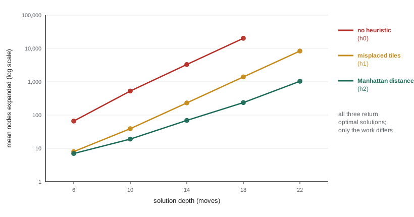
Every run returns a solution of the correct depth, as admissibility guarantees, but the work differs enormously. At depth 18, uniform-cost search expands about 20,000 nodes, misplaced tiles about 1,400 and Manhattan distance about 240, almost a hundred times fewer than no heuristic at all. The effective branching factor of h2 stays near 1.25 while that of h0 stays near 1.65; raised to the twentieth power, that difference is a factor of several hundred.

Manhattan distance wins because it dominates misplaced tiles: h2(n) ≥ h1(n) for every n, since each misplaced tile is at least one square away. If both heuristics are admissible, the dominating one never expands more nodes (apart from ties), because every node with f(n) < C* is expanded anyway, and a larger h pushes more nodes above C*. If you have several admissible heuristics and none dominates, h(n) = max(h1(n), …, hk(n)) is admissible and dominates them all.

Inventing heuristics

Where do good heuristics come from? The most productive idea is the relaxed problem: remove some constraints from the problem and solve the easier version exactly. The cost of an optimal solution to a relaxed problem is an admissible heuristic for the original, because the original's solutions are also solutions of the relaxed problem. It is also consistent, because it is an exact cost in a problem with the same actions plus extras.

Route-finding heuristics come from the relaxation that we can fly in a straight line. Planning heuristics in lesson 11 come from relaxations that ignore preconditions or delete effects. Pattern databases take another approach: they store the exact solution cost of every configuration of a subset of tiles (say tiles 1 to 4 and the blank), computed once by searching backward from the goal, and look it up during search. Disjoint pattern databases, whose subsets do not share tiles and which count only the moves of their own tiles, can be added together and remain admissible; they solve random 15-puzzles in milliseconds. Heuristics can also be learned from data, which is one way neural networks enter search, as in the value networks of AlphaGo in lesson 5.

Memory-bounded search: IDA*

A* keeps every generated node in memory, so on large problems it runs out of memory before it runs out of time, just as BFS does. Iterative deepening A* (IDA*), introduced by Richard Korf in 1985, applies the idea of iterative deepening to f costs. Each iteration is a depth-first search that prunes any node whose f exceeds the current bound; the next bound is the smallest f that exceeded the previous one. With an admissible heuristic IDA* is optimal, and its memory is linear in the solution depth.

# IDA*: depth-first search with an f = g + h cost bound that grows each iteration.
GOAL = (1, 2, 3, 4, 5, 6, 7, 8, 0)
ADJ = {i: [j for j in (i - 3, i + 3, i - 1, i + 1)
           if 0 <= j < 9 and (j // 3 == i // 3 or j % 3 == i % 3)] for i in range(9)}
POS = {t: divmod(i, 3) for i, t in enumerate(GOAL)}
def manhattan(s):
    return sum(abs(i // 3 - POS[t][0]) + abs(i % 3 - POS[t][1]) for i, t in enumerate(s) if t)

def ida_star(start):
    bound, expanded = manhattan(start), 0
    path = [start]
    def search(g, bound):
        nonlocal expanded
        s = path[-1]; f = g + manhattan(s)
        if f > bound: return f                        # report the smallest f that exceeded the bound
        if s == GOAL: return "found"
        expanded += 1; smallest = float("inf")
        i = s.index(0)
        for j in ADJ[i]:
            t = list(s); t[i], t[j] = t[j], t[i]; t = tuple(t)
            if len(path) > 1 and t == path[-2]: continue   # do not undo the last move
            path.append(t)
            r = search(g + 1, bound)
            if r == "found": return r
            smallest = min(smallest, r); path.pop()
        return smallest
    while True:
        r = search(0, bound)
        print(f"  bound {bound:2}: total expanded so far {expanded:7,}")
        if r == "found": return len(path) - 1, expanded
        bound = r

hardest = (8, 6, 7, 2, 5, 4, 3, 0, 1)                 # one of the two 31-move instances
moves, n = ida_star(hardest)
print("solution length", moves, "with", f"{n:,}", "expansions and memory for one path only")

  bound 21: total expanded so far       3
  bound 23: total expanded so far      45
  bound 25: total expanded so far     294
  bound 27: total expanded so far   2,361
  bound 29: total expanded so far  13,455
  bound 31: total expanded so far  14,195
solution length 31 with 14,195 expansions and memory for one path only

Because each iteration repeats the previous ones, IDA* works best when f values are integers that grow in a few large steps, as in the sliding-tile puzzles (in the 8-puzzle the bound rises by 2 each time, because every move changes the Manhattan distance by exactly 1 and the parity of f never changes). When costs are real numbers and nearly every node has a distinct f, IDA* might add only one node per iteration. Other memory-bounded algorithms, such as recursive best-first search and simplified memory-bounded A* (SMA*), use whatever memory is available and discard the least promising nodes when it fills up.

Weighted A* and other satisficing searches

Sometimes a good solution found quickly is better than an optimal solution found slowly. Weighted A* inflates the heuristic: it expands nodes in order of f(n) = g(n) + w·h(n) with w > 1. It behaves more greedily as w grows, and with an admissible h it is bounded suboptimal: its solution costs at most w times the optimal cost. The experiment below runs weighted A* on 30 seeded instances of depth 24.

# Weighted A*: f = g + w*h trades solution quality for speed (seeded 8-puzzle instances at depth 24).
import heapq, random
from collections import deque
GOAL = (1, 2, 3, 4, 5, 6, 7, 8, 0)
ADJ = {i: [j for j in (i - 3, i + 3, i - 1, i + 1)
           if 0 <= j < 9 and (j // 3 == i // 3 or j % 3 == i % 3)] for i in range(9)}
POS = {t: divmod(i, 3) for i, t in enumerate(GOAL)}
def successors(s):
    i = s.index(0)
    for j in ADJ[i]:
        t = list(s); t[i], t[j] = t[j], t[i]; yield tuple(t)
def h(s): return sum(abs(i // 3 - POS[t][0]) + abs(i % 3 - POS[t][1]) for i, t in enumerate(s) if t)

def weighted_astar(start, w):
    frontier, g, expanded = [(w * h(start), 0, start)], {start: 0}, 0
    while frontier:
        _, gs, s = heapq.heappop(frontier)
        if s == GOAL: return gs, expanded
        if gs > g[s]: continue
        expanded += 1
        for t in successors(s):
            if gs + 1 < g.get(t, 99):
                g[t] = gs + 1; heapq.heappush(frontier, (gs + 1 + w * h(t), gs + 1, t))

depth, q = {GOAL: 0}, deque([GOAL])
while q:
    s = q.popleft()
    for t in successors(s):
        if t not in depth: depth[t] = depth[s] + 1; q.append(t)
pool = sorted(s for s, d in depth.items() if d == 24)
sample = random.Random(366).sample(pool, 30)
for w in (1.0, 1.5, 2.0, 3.0, 10.0):
    runs = [weighted_astar(s, w) for s in sample]
    cost = sum(c for c, _ in runs) / len(runs); nodes = sum(n for _, n in runs) / len(runs)
    print(f"w = {w:4}: mean expanded {nodes:7,.0f}   mean cost {cost:5.2f}   worst ratio to optimal {max(c for c, _ in runs) / 24:.2f}")

w =  1.0: mean expanded   1,869   mean cost 24.00   worst ratio to optimal 1.00
w =  1.5: mean expanded     724   mean cost 24.60   worst ratio to optimal 1.17
w =  2.0: mean expanded     589   mean cost 25.53   worst ratio to optimal 1.33
w =  3.0: mean expanded     511   mean cost 28.47   worst ratio to optimal 1.50
w = 10.0: mean expanded     359   mean cost 39.67   worst ratio to optimal 2.33

With w = 1.5 the search expands less than half as many nodes and the average solution is only 2.5 per cent longer than optimal; the worst case stays well inside the guaranteed bound of 1.5. As w grows, the search approaches greedy best-first search: still faster, with much longer solutions. Video games, robotics and the planners of lesson 11 use weighted A* and anytime variants that find a quick solution with a large w and then keep improving it while time remains.

Worked examples