Constraint satisfaction problems

The search algorithms so far treat a state as a black box: a goal test says yes or no, and a successor function generates neighbours, but the algorithm cannot look inside. Many problems have a more useful structure. A state is an assignment of values to variables, and the goal is any assignment that satisfies a set of constraints. Exam timetables, sports schedules, crew rosters, product configurations, Sudoku and map colouring all fit this pattern. Constraint satisfaction problems (CSPs) exploit that structure with general-purpose methods: inference that prunes impossible values before trying them, and variable and value ordering heuristics that steer the search. The results are often dramatic, turning problems that are hopeless for blind search into instant ones.

This lesson defines CSPs, develops backtracking search with the standard heuristics, covers constraint propagation with forward checking and the AC-3 arc-consistency algorithm, applies them to map colouring and Sudoku, and then shows min-conflicts local search and the special case of tree-structured problems. Industrial constraint solvers, and the closely related SAT solvers of lesson 7 and integer programming, schedule airlines, sports leagues and factories every day.

Defining a CSP

A constraint satisfaction problem has three components: a set of variables X1, …, Xn; for each variable a domain Di of possible values; and a set of constraints, each of which restricts the combinations of values that some subset of variables may take. A complete assignment gives every variable a value; a consistent assignment violates no constraint; a solution is a complete, consistent assignment. Some problems also include preferences (soft constraints), turning the CSP into a constrained optimization problem.

Map colouring is the classic example. The variables are the 13 provinces and territories, each domain is a set of colours such as {red, green, blue}, and for every pair of regions that share a land border there is a binary constraint that their colours differ: British Columbia ≠ Alberta, Alberta ≠ Saskatchewan, and so on, 15 constraints in all. Prince Edward Island has no land border, so it is unconstrained. The constraint graph has a node for each variable and an edge for each binary constraint.

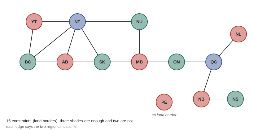
Constraints come in several kinds. A unary constraint restricts one variable (Nunavut is not red); a binary constraint relates two; a higher-order or global constraint relates many. The most common global constraint is AllDiff, which says that a set of variables must all take different values; each row, column and box of a Sudoku grid is an AllDiff over nine cells. Any finite-domain CSP can be translated into one with only binary constraints, but solvers usually keep global constraints, because specialized algorithms for them prune more effectively.

Backtracking search

We could solve a CSP with the search algorithms of lesson 2, treating a partial assignment as a state and 'assign a value to some unassigned variable' as an action. With n variables and domain size d, though, the branching factor at the top would be nd, then (n − 1)d and so on, giving n!·d^n leaves when there are only d^n possible assignments. The key observation is commutativity: the order in which we assign variables does not matter for the final assignment. So we need consider only one variable at each node of the search tree, which cuts the leaves to d^n.

Backtracking search is depth-first search over partial assignments that chooses one variable at each level, tries its values in turn, checks each against the constraints with the variables already assigned, and backtracks as soon as no value is consistent. Plain backtracking is often slow because it makes uninformed choices. Three questions guide improvements: which variable to assign next, in which order to try its values, and what inferences to draw after each assignment.

Variable and value ordering

The minimum-remaining-values (MRV) heuristic chooses the variable with the fewest legal values left. It is called the fail-first heuristic, because it picks the variable most likely to cause a failure soon, pruning the tree early; if some variable has no legal values left, MRV selects it at once and the search backtracks without wasted work. To break ties, especially at the start when all domains are full, the degree heuristic chooses the variable involved in the most constraints with other unassigned variables.

Once a variable is chosen, the least-constraining-value (LCV) heuristic tries first the value that rules out the fewest choices for neighbouring variables. Note the asymmetry: for variables we fail first, for values we fail last. The reason is that every variable must be assigned eventually, so it pays to find out early that the current path is doomed; but we only need one value to work, so we try the most promising first. When we want all solutions, or the problem has none, value ordering does not matter.

Forward checking and arc consistency

Inference can prune domains as search proceeds. Forward checking is the simplest form: whenever a variable X is assigned, for each unassigned variable Y connected to X by a constraint, delete from Y's domain any value inconsistent with X's value. If some domain becomes empty, backtrack immediately. Combined with MRV, forward checking is very effective, because the pruned domain sizes are exactly what MRV needs.

# Colouring the map of the provinces and territories as a constraint satisfaction problem.
BORDERS = """BC-AB BC-YT BC-NT AB-SK AB-NT SK-MB SK-NT MB-ON MB-NU ON-QC QC-NB QC-NL NB-NS YT-NT NT-NU"""
ISLANDS = ["PE"]                      # no land border; any colour works
PALETTE = ["red", "green", "blue", "yellow"]

ADJACENT = {}
for pair in BORDERS.split():
    a, b = pair.split("-")
    ADJACENT.setdefault(a, set()).add(b); ADJACENT.setdefault(b, set()).add(a)
for r in globals().get("ISLANDS", []): ADJACENT[r] = set()
REGIONS = sorted(ADJACENT)

class GiveUp(Exception): pass

def backtrack(k, smart, budget=100000):
    """Return (solution, None, or "gave up"; number of assignments tried)."""
    domains = {r: list(range(k)) for r in REGIONS}
    tries = 0
    def consistent(r, v, a): return all(a.get(n) != v for n in ADJACENT[r])
    def solve(a, domains):
        nonlocal tries
        if len(a) == len(REGIONS): return dict(a)
        free = [r for r in REGIONS if r not in a]
        if smart:   # MRV, ties broken by degree (most constraints on other free regions)
            r = min(free, key=lambda r: (len(domains[r]), -sum(n not in a for n in ADJACENT[r]), r))
        else:
            r = free[0]
        for v in domains[r]:
            if not consistent(r, v, a): continue
            tries += 1; a[r] = v
            if tries > budget: raise GiveUp
            if smart:   # forward checking: remove v from free adjacent regions, fail early on a wipe-out
                pruned = {n: [x for x in domains[n] if x != v] if n in ADJACENT[r] and n not in a else domains[n] for n in domains}
                if all(pruned[n] for n in REGIONS if n not in a):
                    result = solve(a, pruned)
                    if result: return result
            else:
                result = solve(a, domains)
                if result: return result
            del a[r]
        return None
    try:
        return solve({}, domains), tries
    except GiveUp:
        return "gave up", budget

print(len(REGIONS), "regions,", sum(len(v) for v in ADJACENT.values()) // 2, "borders")
first = None
for k in (2, 3, 4):
    for smart in (False, True):
        sol, tries = backtrack(k, smart)
        name = "MRV + degree + forward checking" if smart else "plain backtracking            "
        outcome = sol if sol == "gave up" else ("solved" if sol else "no solution")
        print(f"{k} labels, {name}: {outcome} after {tries:,} assignments")
        if isinstance(sol, dict) and first is None: first = sol
print("first solution:", ", ".join(f"{r} {PALETTE[v]}" for r, v in sorted(first.items())))

13 regions, 15 borders
2 labels, plain backtracking            : no solution after 48 assignments
2 labels, MRV + degree + forward checking: no solution after 4 assignments
3 labels, plain backtracking            : solved after 13 assignments
3 labels, MRV + degree + forward checking: solved after 13 assignments
4 labels, plain backtracking            : solved after 13 assignments
4 labels, MRV + degree + forward checking: solved after 13 assignments
first solution: AB red, BC green, MB red, NB red, NL red, NS green, NT blue, NU green, ON green, PE red, QC blue, SK green, YT red

The Canadian map is easy: its constraint graph is sparse and almost a tree, so plain backtracking already colours it with three colours after one assignment per region, and forward checking proves two colours impossible after only 4 assignments rather than 48. The value of the heuristics shows on larger, denser graphs. On the 48 contiguous states, with 105 borders, plain backtracking in alphabetical order gives up after 100,000 assignments when asked for three colours, while MRV with forward checking proves in 99 assignments that three colours cannot work, because Nevada's five neighbours form a ring of odd length. With four colours, the heuristics cut the work from 4,957 assignments to 48, one per state.

Forward checking looks only one step ahead, from the assigned variable to its neighbours. Arc consistency looks further. A variable X is arc-consistent with respect to Y if for every value in X's domain there is some value in Y's domain that satisfies the binary constraint between them; such a value is called a support. A CSP is arc-consistent if every variable is arc-consistent with respect to every other. The AC-3 algorithm (Mackworth, 1977, developed at the University of British Columbia) enforces arc consistency. It keeps a queue of arcs (X, Y). For each arc it removes from X's domain every value with no support in Y; if X's domain shrank, every arc (Z, X) pointing into X goes back on the queue, because a value of Z might have lost its only support. If a domain becomes empty, the CSP has no solution.

With n variables, c binary constraints and domain size at most d, AC-3 runs in O(cd³) time: each arc can be added to the queue at most d times (once per value deleted from its target), and checking an arc costs O(d²). Arc consistency can be enforced before search starts, as a preprocessing step, or after every assignment, which is called maintaining arc consistency (MAC) and detects failures that forward checking misses. Stronger forms exist: path consistency considers triples of variables, and k-consistency considers any k; they prune more but cost more, and in practice arc consistency or a little more is the usual compromise.

Sudoku: propagation and search together

Sudoku is a good showcase for combining inference with search. The program below represents each cell's domain as a set of digits, enforces arc consistency with AC-3 on the binary 'differs from' constraints between peers (cells sharing a row, column or box), and if that does not finish the puzzle, chooses a cell by MRV, tries its values, and runs AC-3 again after each choice.

# Sudoku as a CSP: AC-3 constraint propagation, then backtracking search with MRV.
from collections import deque
PUZZLES = {
 "easy": "530070000600195000098000060800060003400803001700020006060000280000419005000080079",
 "hard": "000000010400000000020000000000050407008000300001090000300400200050100000000806000",
}
CELLS = [(r, c) for r in range(9) for c in range(9)]
PEERS = {(r, c): {(i, j) for (i, j) in CELLS if (i, j) != (r, c) and
                  (i == r or j == c or (i // 3, j // 3) == (r // 3, c // 3))} for (r, c) in CELLS}

def ac3(dom):
    """Make every arc X != Y consistent. Returns False if some domain becomes empty."""
    queue = deque((x, y) for x in CELLS for y in PEERS[x])
    while queue:
        x, y = queue.popleft()
        if len(dom[y]) == 1 and dom[y] <= dom[x]:            # x has no support for the value y must take
            dom[x] = dom[x] - dom[y]
            if not dom[x]: return False
            queue.extend((z, x) for z in PEERS[x] if z != y)
    return True

stats = {"assignments": 0}
def search(dom):
    if not ac3(dom): return None
    if all(len(d) == 1 for d in dom.values()): return dom
    cell = min((c for c in CELLS if len(dom[c]) > 1), key=lambda c: (len(dom[c]), c))   # MRV
    for v in sorted(dom[cell]):
        stats["assignments"] += 1
        trial = {c: set(d) for c, d in dom.items()}; trial[cell] = {v}
        result = search(trial)
        if result: return result
    return None

for name, p in PUZZLES.items():
    dom = {c: {int(p[9 * c[0] + c[1]])} if p[9 * c[0] + c[1]] != "0" else set(range(1, 10)) for c in CELLS}
    given = sum(ch != "0" for ch in p)
    after = {c: set(d) for c, d in dom.items()}; ac3(after)
    fixed = sum(len(d) == 1 for d in after.values())
    stats["assignments"] = 0
    sol = search(dom)
    print(f"{name}: {given} givens; AC-3 alone fixes {fixed} of 81 cells; search made {stats['assignments']} guesses")
    if name == "easy":
        for r in range(9): print("   ", " ".join(str(next(iter(sol[(r, c)]))) for c in range(9)))

easy: 30 givens; AC-3 alone fixes 81 of 81 cells; search made 0 guesses
    5 3 4 6 7 8 9 1 2
    6 7 2 1 9 5 3 4 8
    1 9 8 3 4 2 5 6 7
    8 5 9 7 6 1 4 2 3
    4 2 6 8 5 3 7 9 1
    7 1 3 9 2 4 8 5 6
    9 6 1 5 3 7 2 8 4
    2 8 7 4 1 9 6 3 5
    3 4 5 2 8 6 1 7 9
hard: 17 givens; AC-3 alone fixes 18 of 81 cells; search made 1456 guesses

For the easy puzzle, a typical newspaper Sudoku with 30 givens, arc consistency alone determines every cell; no search is needed. The hard puzzle has only 17 givens, the minimum number for a puzzle with a unique solution, and AC-3 fixes just one cell beyond the givens. Search with MRV and propagation then solves it after about 1,500 guesses, in well under a second. Stronger inference on the AllDiff constraints, such as the 'naked pairs' and 'hidden singles' that experienced human solvers use, would shrink the search further; each is a special case of a more general consistency algorithm.

Intelligent backtracking

When plain backtracking hits a dead end it returns to the most recently assigned variable, which may have nothing to do with the failure. Conflict-directed backjumping keeps, for each variable, a conflict set: the earlier assignments that ruled out its values. On failure it jumps back to the most recent variable in the conflict set, skipping irrelevant ones. Constraint learning goes further and records the combination of assignments that caused the failure as a new constraint, a nogood, so the same mistake is never repeated elsewhere in the tree. Learned nogoods are the heart of modern SAT solvers, as lesson 7 explains.

Local search for CSPs: min-conflicts

Local search from lesson 4 also suits CSPs. Start with a complete assignment that violates some constraints; repeatedly pick a variable in conflict at random and change it to the value that violates the fewest constraints, breaking ties at random. This min-conflicts heuristic is astonishingly effective on some problems. On n-queens its running time is roughly independent of n once a reasonable initial assignment is made, because solutions are densely spread through the space.

# Min-conflicts local search for n-queens (one queen per column), seeded.
import random

def min_conflicts(n, rng, max_steps=100000):
    rows = [0] * n
    row_count, d1, d2 = [0] * n, [0] * (2 * n), [0] * (2 * n)
    def place(c, r, delta):
        row_count[r] += delta; d1[r + c] += delta; d2[r - c + n] += delta
    for c in range(n):                       # greedy start: each queen on a least-conflicted row
        best = min(range(n), key=lambda r: (row_count[r] + d1[r + c] + d2[r - c + n], rng.random()))
        rows[c] = best; place(c, best, +1)
    def conflicts(c, r): return row_count[r] + d1[r + c] + d2[r - c + n] - 3 * (rows[c] == r)
    for step in range(max_steps):
        bad = [c for c in range(n) if conflicts(c, rows[c]) > 0]
        if not bad: return rows, step
        c = rng.choice(bad)                                    # a conflicted variable at random
        place(c, rows[c], -1)
        scores = [row_count[r] + d1[r + c] + d2[r - c + n] for r in range(n)]
        low = min(scores)
        rows[c] = rng.choice([r for r in range(n) if scores[r] == low])   # value with fewest conflicts
        place(c, rows[c], +1)
    return None, max_steps

for n in (8, 100, 1000):
    steps = [min_conflicts(n, random.Random(seed))[1] for seed in range(5)]
    print(f"n = {n:5}: repair steps to a solution over 5 seeds: {steps}")

n =     8: repair steps to a solution over 5 seeds: [20, 9, 1, 79, 19]
n =   100: repair steps to a solution over 5 seeds: [16, 103, 26, 51, 15]
n =  1000: repair steps to a solution over 5 seeds: [31, 61, 73, 38, 47]

A thousand queens take a few dozen repairs after a greedy start, roughly the same as eight queens. Min-conflicts was made famous by scheduling observations for the Hubble Space Telescope, where it cut the time to schedule a week of observations from three weeks to around ten minutes. Local search also adapts gracefully to change: when a constraint is added (a pilot calls in sick, a room becomes unavailable), it repairs the current schedule rather than starting over, which tends to keep most of the old schedule intact, an important property when people have already made plans around it.

The structure of problems

The structure of the constraint graph can make a CSP easy. If the graph splits into independent components, each can be solved separately: Prince Edward Island never interacts with the rest of the map, and a problem made of components of c variables each costs O(d^c) per component rather than O(d^n) overall. If the graph is a tree, the problem can be solved in O(nd²) time, linear in the number of variables. Choose a root, order the variables so each comes after its parent, make each parent arc-consistent with its child working backward from the leaves, and then assign values forward from the root; arc consistency guarantees a consistent value always remains.

General graphs can be brought closer to trees. Cutset conditioning finds a small set of variables, the cycle cutset, whose removal leaves a tree; it tries each assignment of the cutset and solves the remaining tree, costing O(d^c · (n − c)d²) for a cutset of size c. Tree decomposition groups variables into overlapping clusters arranged in a tree and solves each cluster as a mega-variable; its cost is exponential only in the size of the largest cluster, called the treewidth. These ideas return in lesson 9, where the cost of exact probabilistic inference also depends on the structure of a graph.

Worked examples