Amortized analysis

Some data structures have operations that are usually cheap but occasionally very expensive. A dynamic array appends in constant time until it fills, then copies everything into a larger array. Analysing each operation by its worst case gives a misleadingly pessimistic bound: n appends, each costing up to n, suggests Θ(n²) total, when the true total is Θ(n). Amortized analysis bounds the total cost of any sequence of operations, then spreads it evenly, so that each operation is charged its share. Unlike average-case analysis, it makes no assumptions about the inputs and involves no probability; it is a worst-case guarantee about sequences.

Amortized bounds matter wherever a system processes long streams of operations, which describes most of Northway's server. The ingest buffer grows as records arrive, the union-find structure that merges duplicate node identities runs millions of operations a night, and the rate limiter on the public reporting API decides each second whether to accept a request. This lesson develops three methods for proving amortized bounds, aggregate analysis, the accounting method and the potential method, and applies them to dynamic arrays, binary counters, union-find and a queue built from two stacks.

Aggregate analysis

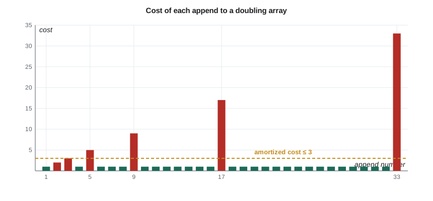
The simplest method computes the total cost T(n) of the worst sequence of n operations directly and divides by n. Consider a dynamic array that starts with capacity 1 and doubles its capacity whenever it is full. Appending to a non-full array costs 1. Appending to a full array of size k costs k to copy the existing elements plus 1 for the new one. Over n appends, the copies happen at sizes 1, 2, 4, …, up to the largest power of two below n, and those copy costs sum to less than 2n. Adding the n unit costs gives fewer than 3n operations in total, so the amortized cost per append is at most 3, a constant.

The growth factor matters. Growing by a constant amount, say 100 slots each time, makes the copies cost 100 + 200 + 300 + … , which is Θ(n²/100), still quadratic. Any constant multiplicative factor greater than 1 gives linear total cost. Python's list grows by about one eighth plus a little, trading more frequent copies for less wasted memory; C++ standard library implementations typically double or grow by 1.5.

The accounting method

The accounting method charges each operation a fixed amortized cost, which may be more or less than its actual cost. When the charge exceeds the actual cost, the difference is stored as credit attached to specific parts of the data structure. When an operation costs more than its charge, it spends stored credit. The method works if the credit never goes negative, because then the total charges are an upper bound on the total actual cost.

For the dynamic array, charge 3 for each append. One unit pays for writing the new element. The other two are stored as credit on the element. When the array of capacity k fills, the k/2 elements added since the last resize each carry 2 credits, giving k credits in total, exactly enough to pay for copying all k elements. The credit never goes negative, so every append is O(1) amortized.

A binary counter illustrates the same idea. Northway's nodes keep a hardware counter of detected vehicles that increments by flipping bits. An increment flips trailing ones to zero and one zero to one, so incrementing from 0111 1111 to 1000 0000 flips eight bits. Charge 2 for each increment: one pays for setting the single bit that becomes 1, and the other is stored on that bit to pay for resetting it to 0 later. Every 1 bit carries one credit, so the cost of clearing trailing ones is always prepaid, and n increments flip at most 2n bits in total.

The potential method

The potential method is the most general. It defines a potential function Φ that maps each state of the data structure to a non-negative number, starting at zero, like stored energy. The amortized cost of an operation is its actual cost plus the change in potential it causes. Summing over a sequence, the potential changes telescope, so the total amortized cost equals the total actual cost plus the final potential, which is non-negative. Total amortized cost is therefore an upper bound on total actual cost.

For the doubling array with n elements and capacity k, take Φ = 2n − k, which is zero just after a resize (when n = k/2) and rises to k just before the next one. A normal append costs 1 and raises Φ by 2, for an amortized cost of 3. A resizing append when n = k costs k + 1, and afterwards the capacity is 2k with n + 1 elements, so Φ changes from 2k − k = k to 2(k + 1) − 2k = 2, a drop of k − 2. The amortized cost is (k + 1) − (k − 2) = 3. Every append costs 3 amortized.

Choosing the potential is the creative step. A good potential is high when the structure is close to an expensive operation and low just after one; it measures how much work has been deferred. For the binary counter, the number of 1 bits works; for a dynamic array, the fullness beyond half; for splay trees, the sum of logarithms of subtree sizes.

Shrinking without thrashing

Dana's ingest buffer also needs to shrink after a burst of uploads, or it holds gigabytes of memory all day. Halving the array whenever it becomes half full looks symmetric but is a trap: an array that has just doubled to capacity 2k with k + 1 elements, then loses two elements and halves, then gains two and doubles, pays Θ(k) on every operation. The fix is hysteresis: double when full, but halve only when the array is a quarter full. Then at least k/4 cheap operations separate any two resizes, and the potential method shows every operation is O(1) amortized for any mix of appends and removals.

# Measure total copy cost for doubling growth, constant growth, and naive halving
def run(ops, grow, shrink_at):
    cap, n, cost = 1, 0, 0
    for op in ops:
        if op == '+':
            if n == cap:
                cost += n; cap = grow(cap)
            n += 1; cost += 1
        else:
            n -= 1; cost += 1
            if cap > 1 and n <= cap * shrink_at:
                cost += n; cap //= 2
    return cost

appends = ['+'] * 100000
print("doubling, 100000 appends:", run(appends, lambda c: 2 * c, 0), "operations")
print("grow by 100, 100000 appends:", run(appends, lambda c: c + 100, 0), "operations")

# a burst then oscillation around a power of two
burst = ['+'] * 1025 + ['-', '-', '+', '+'] * 5000
print("halve at 1/2 full, oscillating:", run(burst, lambda c: 2 * c, 0.5), "operations")
print("halve at 1/4 full, oscillating:", run(burst, lambda c: 2 * c, 0.25), "operations")

doubling, 100000 appends: 231071 operations
grow by 100, 100000 appends: 50051000 operations
halve at 1/2 full, oscillating: 10263072 operations
halve at 1/4 full, oscillating: 23072 operations

The oscillating sequence makes the point concrete. With halving at one half, every pair of removals and appends straddles the resize boundary and copies about a thousand elements, so about twenty-one thousand operations cost over ten million. With halving at one quarter, the same sequence costs about twenty-three thousand. The difference is a single constant in the code, and only amortized analysis explains why it matters.

A queue from two stacks

Some message brokers implement a first-in first-out queue with two last-in first-out stacks, because stacks are simpler to make lock-free. Push to the inbox stack. To pop, take from the outbox stack; if it is empty, first move every element from the inbox to the outbox, which reverses their order so the oldest is on top. A single pop can cost Θ(n), but each element is moved from inbox to outbox at most once in its life. Charging 3 per push, one for the push, one for the later move and one for the later pop, shows that every operation is O(1) amortized.

Union-find

Northway's identity service merges records that belong to the same physical node, because nodes are sometimes re-flashed with new identifiers and their history must be joined. The union-find, or disjoint-set, structure maintains a partition of elements into sets, with two operations: find returns a representative of an element's set, and union merges two sets. Each set is a tree whose root is the representative, and find follows parent pointers to the root.

Two simple heuristics make it remarkably fast. Union by rank attaches the shorter tree under the taller one, which keeps trees of height O(log n). Path compression makes every node visited by a find point directly to the root, flattening the tree for future finds. With both, Tarjan proved in 1975 that any sequence of m operations on n elements takes O(m·α(n)) time, where α is the inverse Ackermann function. That function grows so slowly that α(n) ≤ 4 for any n that could fit in the observable universe, so union-find operations are constant time amortized for every practical purpose. Kruskal's minimum spanning tree algorithm in CMPUT-204 relies on exactly this structure.

# Union-find with union by rank and path compression, merging re-flashed node IDs
class DSU:
    def __init__(self):
        self.parent, self.rank, self.steps = {}, {}, 0
    def find(self, x):
        self.parent.setdefault(x, x); self.rank.setdefault(x, 0)
        root = x
        while self.parent[root] != root:
            root = self.parent[root]; self.steps += 1
        while self.parent[x] != root:            # path compression
            self.parent[x], x = root, self.parent[x]
        return root
    def union(self, a, b):
        ra, rb = self.find(a), self.find(b)
        if ra == rb:
            return
        if self.rank[ra] < self.rank[rb]:
            ra, rb = rb, ra
        self.parent[rb] = ra
        if self.rank[ra] == self.rank[rb]:
            self.rank[ra] += 1

d = DSU()
same = [('NS4-0213', 'NS4-0890'), ('NS4-0890', 'NS4-1177'), ('NS4-0042', 'NS4-0315'),
        ('NS4-1177', 'NS4-2004'), ('NS4-0315', 'NS4-0042')]
for a, b in same:
    d.union(a, b)
print("NS4-0213 and NS4-2004 same device:", d.find('NS4-0213') == d.find('NS4-2004'))
print("NS4-0213 and NS4-0042 same device:", d.find('NS4-0213') == d.find('NS4-0042'))

big = DSU()
seed = 99
for _ in range(200000):
    seed = (1103515245 * seed + 12345) % 2**31; a = seed % 100000
    seed = (1103515245 * seed + 12345) % 2**31; b = seed % 100000
    big.union(a, b)
print("pointer steps per operation over 200000 random unions:", round(big.steps / 400000, 2))

NS4-0213 and NS4-2004 same device: True
NS4-0213 and NS4-0042 same device: False
pointer steps per operation over 200000 random unions: 0.87

Amortized versus real-time guarantees

An amortized bound promises a good total, not a good maximum. For a batch job, such as the nightly ingest, that is exactly what matters. For a real-time system it may not be: Maren's firmware samples the radar every 2 milliseconds, and an append that suddenly copies 8,000 records could miss a deadline even though the average cost is tiny. Real-time systems therefore preallocate fixed-size ring buffers, as CMP-200 described, or use incremental resizing that moves a few elements on every operation instead of all at once, converting the amortized bound into a worst-case one at the cost of complexity. CMP-440 Real-Time Systems returns to this trade-off.