
CMP-301 · Lesson 12 of 12 · 21 min
Coping with hardness and capstone: scheduling sensor uploads
An NP-completeness proof does not make a problem go away. Northway still has to place gateways, route the field crew and schedule uploads, and customers still expect answers by morning. This final lesson surveys what engineers do when a problem is NP-hard: exploit special structure, run exact algorithms that are exponential only in a small parameter, accept answers with a proven approximation guarantee, use heuristics that work well in practice, or hand the problem to an industrial solver. It ends with the capstone that has run through the course, Dana's upload scheduling problem, where the main lesson is that the right formulation can make a problem that looks hard turn out to be easy.
Strategy 1: look for special structure
Hardness results are about the general problem. The instance in front of you may have structure that makes it easy. Vertex cover is NP-hard on general graphs but linear on trees, as lesson 5 showed, and polynomial on bipartite graphs, by König's theorem and maximum matching from lesson 6. 2-SAT is linear. Colouring an interval graph, such as assigning radio channels to time windows, is solved greedily. Knapsack with small capacities is solved by dynamic programming. Before reaching for heavy machinery, ask whether the real inputs are trees, bipartite, planar, small in some dimension, or have small numbers.
Strategy 2: exact algorithms that are fast enough
Exponential does not always mean impossible. Branch and bound searches the tree of partial solutions but prunes any branch whose best possible completion cannot beat the best solution found so far. With good bounds it solves TSP instances with thousands of cities exactly. Modern integer linear programming (ILP) solvers combine branch and bound with cutting planes and clever heuristics and routinely solve industrial scheduling problems with hundreds of thousands of variables. SAT solvers based on conflict-driven clause learning handle formulas with millions of clauses from hardware verification. These tools have worst-case exponential running times, but on real instances they often finish in seconds, and they are the first thing to try when an exact answer matters.
Parameterized algorithms make the exponential part depend only on a parameter that is small in practice. Vertex cover of size k can be decided in O(2ᵏ·n) time: pick any uncovered edge; one of its two endpoints must be in the cover, so branch on both, each time reducing k by one. The search tree has at most 2ᵏ leaves. For Maren's relay problem on a general mesh, where the cover is known to have at most about 15 nodes, that is about 33,000 branches, each linear, which is instantaneous even though the problem is NP-hard. Problems with such algorithms are called fixed-parameter tractable.
# Fixed-parameter vertex cover: branch on an uncovered edge, depth at most k
def has_cover(edges, k, chosen=()):
    uncovered = [(u, v) for u, v in edges if u not in chosen and v not in chosen]
    if not uncovered:
        return list(chosen)
    if k == 0:
        return None
    u, v = uncovered[0]
    return has_cover(edges, k - 1, chosen + (u,)) or has_cover(edges, k - 1, chosen + (v,))

mesh = [(1, 2), (1, 3), (2, 4), (3, 4), (4, 5), (5, 6), (5, 7), (6, 8), (7, 8),
        (8, 9), (9, 10), (2, 10), (3, 7)]
for k in range(1, 8):
    c = has_cover(mesh, k)
    print(f"k = {k}: {'cover ' + str(sorted(c)) if c else 'none'}")
    if c:
breakk = 1: none k = 2: none k = 3: none k = 4: none k = 5: cover [2, 3, 5, 8, 9]
Strategy 3: approximation algorithms with guarantees
An approximation algorithm runs in polynomial time and returns a solution provably within a factor of optimal. The approximation ratio of a minimization algorithm is the worst case, over all instances, of its cost divided by the optimal cost. A ratio of 2 means the answer is never more than twice optimal, a guarantee no heuristic offers.
Vertex cover has a simple 2-approximation. Repeatedly take any uncovered edge and put both of its endpoints in the cover. The chosen edges share no endpoints, they form a matching, and any cover must contain at least one endpoint of each, so the optimum has at least as many vertices as the matching has edges. The algorithm takes exactly twice that many. Remarkably, no polynomial algorithm with a ratio below 2 is known, and under a widely believed conjecture none exists.
Set cover, the gateway problem, has a greedy approximation: repeatedly choose the pole that covers the most counters not yet covered. Its ratio is about ln n, where n is the number of counters, and a deep result shows that no polynomial algorithm can do substantially better unless P = NP. In practice greedy is usually within 10 to 20 percent of optimal, and for the 70-pole corridor it found a solution with 9 gateways when an ILP solver later proved 8 optimal.
For TSP, approximation depends on the distances. If they obey the triangle inequality, as road travel times roughly do, doubling a minimum spanning tree and shortcutting repeated vertices gives a tour at most twice optimal, and Christofides' algorithm from 1976 improves the ratio to 1.5 by adding a minimum-weight matching on the odd-degree vertices. Without the triangle inequality no constant-ratio approximation exists unless P = NP, because one would decide Hamiltonian cycle.
Knapsack admits something better, a fully polynomial-time approximation scheme (FPTAS). For any ε > 0, round each value down to a multiple of εv_max/n and run the value-indexed dynamic program on the rounded values. The table is now polynomial in n and 1/ε, and the rounding loses at most a factor (1 − ε). Maren can ask for an answer within 1 percent of optimal and get it in milliseconds even with values in the millions.
| Problem | Best known polynomial guarantee | Method |
|---|---|---|
| Vertex cover | Ratio 2 | Take both ends of a maximal matching |
| Set cover | Ratio about ln n | Greedy: most new elements first |
| Metric TSP | Ratio 1.5 | Christofides (MST plus matching) |
| General TSP | No constant ratio unless P = NP | Use heuristics or exact solvers |
| Knapsack | Within 1 − ε for any ε (FPTAS) | Scaled-value dynamic programming |
| Bin packing | About 11/9 OPT plus a constant | First fit decreasing |
Strategy 4: heuristics and local search
When guarantees are unavailable or too weak, heuristics that perform well in practice fill the gap. Constructive heuristics build a solution greedily, such as nearest neighbour for TSP, always driving to the closest unvisited site. Local search then improves it by small changes. The 2-opt move for TSP removes two edges of the tour and reconnects the pieces the other way, which uncrosses crossing routes; repeating until no move helps typically gives tours within about 5 percent of optimal. Metaheuristics such as simulated annealing, which sometimes accepts worse moves to escape local minima, and genetic algorithms extend local search further. The Lin-Kernighan heuristic and its descendants find tours within a fraction of a percent of optimal on instances with millions of cities.
# Nearest-site tour, then 2-opt for the 38-site calibration route (deterministic sites)
import math
seed, sites = 31, [(0.0, 0.0)]                    # depot at the origin, km on a grid
for _ in range(38):
    seed = (1103515245 * seed + 12345) % 2**31; x = (seed % 4000) / 100 - 20
    seed = (1103515245 * seed + 12345) % 2**31; y = (seed % 4000) / 100 - 20
    sites.append((x, y))
dist = lambda a, b: math.dist(sites[a], sites[b])
length = lambda t: sum(dist(t[i], t[(i + 1) % len(t)]) for i in range(len(t)))

tour, left = [0], set(range(1, len(sites)))
while left:
    nxt = min(left, key=lambda j: dist(tour[-1], j)); tour.append(nxt); left.remove(nxt)
print(f"nearest site: {length(tour):6.1f} km")

improved = True
while improved:
    improved = False
    for i in range(1, len(tour) - 1):
        for j in range(i + 1, len(tour)):
            a, b, c, d = tour[i - 1], tour[i], tour[j], tour[(j + 1) % len(tour)]
            if dist(a, c) + dist(b, d) < dist(a, b) + dist(c, d) - 1e-9:
                tour[i:j + 1] = reversed(tour[i:j + 1]); improved = True
print(f"after 2-opt: {length(tour):6.1f} km")nearest site: 247.3 km after 2-opt: 194.9 km
The capstone: scheduling sensor uploads
Return now to the problem Jonah formulated in lesson 1. Each night every node has one data batch ready at a release time r_j and due at a deadline d_j. The night is divided into 15-minute slots. The carrier's price varies by slot, cheap after midnight and expensive near dawn when other customers' devices wake up, and the server's ingest link can accept at most c uploads in any slot. Assign each batch to a slot between its release and deadline so that no slot exceeds its capacity and the total cost is as small as possible.
At first glance this looks like scheduling with deadlines and capacities, the kind of problem that is often NP-hard. The structure says otherwise. Each batch needs exactly one slot, each slot has an integer capacity, and the cost depends only on the slot. That is a minimum-cost flow problem: a source with an edge of capacity 1 to each batch, an edge of capacity 1 from each batch to each slot in its window, and an edge from each slot to the sink with capacity c and cost equal to the slot's price. By the integrality theorem of lesson 6, extended to minimum-cost flow, an optimal integer flow exists and gives the optimal schedule. Minimum-cost flow is solvable in polynomial time, for example by repeatedly augmenting along the cheapest residual path found with Bellman-Ford, which handles the negative-cost backward edges.
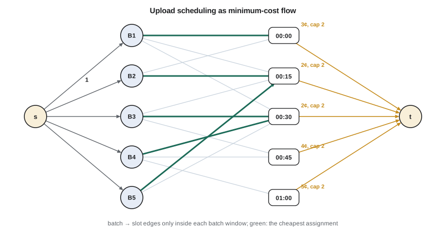
# Capstone: optimal upload schedule by min-cost flow vs a greedy baseline
def min_cost_flow(n, edges, s, t, need):
    graph = [[] for _ in range(n)]
    def add(u, v, cap, cost):
        graph[u].append([v, cap, cost, len(graph[v])])
        graph[v].append([u, 0, -cost, len(graph[u]) - 1])
    for e in edges: add(*e)
    flow = cost = 0
    while flow < need:
        dist, prev = [float('inf')] * n, [None] * n
        dist[s] = 0
        for _ in range(n - 1):                      # Bellman-Ford on the residual graph
            changed = False
            for u in range(n):
                if dist[u] == float('inf'): continue
                for i, (v, cap, c, _) in enumerate(graph[u]):
                    if cap > 0 and dist[u] + c < dist[v]:
                        dist[v] = dist[u] + c; prev[v] = (u, i); changed = True
            if not changed: break
        if dist[t] == float('inf'): return None
        v = t
        while v != s:
            u, i = prev[v]; graph[u][i][1] -= 1
            graph[v][graph[u][i][3]][1] += 1; v = u
        flow += 1; cost += dist[t]
    return cost, graph

slots = ['00:00', '00:15', '00:30', '00:45', '01:00', '01:15']
price = [3, 2, 2, 4, 5, 6]                          # cents per upload in each slot
cap = 2
batches = {'B1': (0, 2), 'B2': (0, 1), 'B3': (1, 3), 'B4': (2, 5), 'B5': (1, 2),
           'B6': (3, 5), 'B7': (0, 5), 'B8': (4, 5)}   # (release slot, deadline slot)
names = list(batches)
S, T = 0, 1 + len(names) + len(slots)
edges = [(S, 1 + j, 1, 0) for j in range(len(names))]
for j, b in enumerate(names):
    r, d = batches[b]
    edges += [(1 + j, 1 + len(names) + k, 1, 0) for k in range(r, d + 1)]
edges += [(1 + len(names) + k, T, cap, price[k]) for k in range(len(slots))]
cost, g = min_cost_flow(T + 1, edges, S, T, len(names))
plan = {names[j]: slots[e[0] - 1 - len(names)] for j in range(len(names))
        for e in g[1 + j] if e[0] > len(names) and e[1] == 0}
print("optimal cost:", cost, "cents ->", dict(sorted(plan.items())))

load, gcost = [0] * len(slots), 0                    # greedy: earliest deadline, cheapest open slot
for b in sorted(names, key=lambda b: batches[b][1]):
    r, d = batches[b]
    k = min((k for k in range(r, d + 1) if load[k] < cap), key=lambda k: price[k])
    load[k] += 1; gcost += price[k]
print("greedy cost: ", gcost, "cents")optimal cost: 23 cents -> {'B1': '00:00', 'B2': '00:15', 'B3': '00:30', 'B4': '00:30', 'B5': '00:15', 'B6': '00:45', 'B7': '00:00', 'B8': '01:00'}
greedy cost: 24 centsOn the eight-batch example the flow model finds the cheapest schedule, and the greedy rule, which handles urgent batches first and puts each in its cheapest open slot, pays more because it fills cheap slots with flexible batches that could have waited. On the real network, 400 nodes and 32 slots, the flow model solves in well under a second and cut the nightly cellular cost by about 18 percent compared with every node uploading at 01:00. Dana's original question, which Jonah feared was NP-hard, turned out to be in P.
The formulation is fragile, though, and the course's two halves meet here. If batches have different sizes and slots have bandwidth limits in megabytes, the problem contains bin packing and becomes NP-hard. If each node can split its batch across several slots, it becomes a linear program, solvable in polynomial time again. If gateways share radio channels so that neighbouring nodes cannot upload in the same slot, graph colouring appears and the problem is hard. The skill this course has tried to build is noticing which of these worlds a problem lives in, choosing the matching tool, and proving that the choice is right.
Worked problem
Approximating a vertex cover
Apply the matching-based 2-approximation to the mesh edges (1,2), (1,3), (2,4), (3,4), (4,5) taking edges in that order, and compare with the optimum.
Show solution
- Take (1,2): add 1 and 2. Edges (1,3) and (2,4) are now covered.
- (3,4) is uncovered: add 3 and 4. Now (4,5) is covered too.
- Approximate cover: {1, 2, 3, 4}, size 4.
- Optimal cover: {1, 4} covers (1,2), (1,3), (2,4), (3,4) and (4,5), size 2.
- Ratio 4/2 = 2, exactly the worst case the guarantee allows.
Answer: The guarantee is tight on this instance, which is typical: approximation ratios are worst-case promises, and real instances usually do better.
Common mistakes
MistakeGiving up on a problem as soon as it is shown NP-hard.
InsteadCheck for special structure, small parameters, approximation guarantees, good heuristics and industrial solvers before deciding it cannot be solved well.
MistakeReporting a heuristic's result as optimal.
InsteadHeuristics carry no guarantee. Compare against a lower bound, an exact solver on small instances or an approximation bound.
MistakeAssuming any scheduling problem with deadlines is NP-hard.
InsteadUnit jobs with slot capacities and slot costs form a minimum-cost flow problem, solvable in polynomial time. Formulate before concluding.
MistakeUsing an approximation ratio from the metric version on a non-metric instance.
InsteadThe 1.5 ratio for TSP needs the triangle inequality; without it no constant ratio is possible unless P = NP.
Summary and key terms
- Special structure, such as trees, bipartite graphs or small numbers, often makes NP-hard problems easy.
- Branch and bound, ILP and SAT solvers solve many large instances exactly despite exponential worst cases.
- Fixed-parameter algorithms, such as O(2ᵏn) vertex cover, are exponential only in a small parameter.
- Approximation algorithms guarantee a ratio: 2 for vertex cover, about ln n for set cover, 1.5 for metric TSP, 1 − ε for knapsack.
- Heuristics such as nearest neighbour with 2-opt work well in practice but carry no guarantee.
- Upload scheduling with unit batches, slot capacities and slot prices is minimum-cost flow and therefore in P; small changes make it NP-hard.
- Approximation algorithm
- A polynomial-time algorithm whose solution is guaranteed within a stated factor of optimal.
- Approximation ratio
- The worst-case ratio of an algorithm’s cost to the optimal cost.
- Fixed-parameter tractable
- Solvable in time f(k)·poly(n), exponential only in a parameter k.
- Branch and bound
- An exact search that prunes partial solutions whose best completion cannot beat the current best.
- FPTAS
- A fully polynomial-time approximation scheme: within 1 − ε of optimal in time polynomial in n and 1/ε.
- 2-opt
- A local search move for tours that removes two edges and reconnects the paths the other way.
- Minimum-cost flow
- Finding a flow of required value whose total edge cost is as small as possible.
Practice problems
Work each problem on paper first, then reveal the answer to check.
A 2-approximation for vertex cover returns 46 vertices. What can you say about the optimum?
Show answer
It has at least 23 vertices and at most 46.
Why does doubling an MST give a TSP tour at most twice optimal under the triangle inequality?
Show answer
Deleting one edge from an optimal tour gives a spanning tree, so the MST weighs at most the optimal tour; walking around the doubled MST costs twice that, and shortcutting repeated vertices does not increase the length.
How many branches does the fixed-parameter vertex cover search explore at most for k = 12?
Show answer
2¹² = 4,096 leaves.
If each upload batch could be split across slots, what kind of problem would scheduling become?
Show answer
A linear program (fractional flow), still solvable in polynomial time.
Lesson quiz · 5 questions
Score 60% or more to complete this lesson.
Create a free account to save your progress, take quizzes and earn a certificate.