
CMP-301 · Lesson 3 of 12 · 19 min
Divide and conquer and the master theorem
Divide and conquer solves a problem by splitting it into smaller independent subproblems of the same kind, solving those recursively, and combining their answers. Merge sort, which you analysed in CMP-200 and CMPUT-204, is the standard example: split the list in half, sort each half, and merge. The paradigm is powerful because a split that halves the problem size turns linear work per level into logarithmic depth, and it often reduces a quadratic brute force to n log n. This lesson examines divide-and-conquer recurrences with the master theorem and applies the paradigm to three problems where the clever part is the combine step: counting inversions, finding the closest pair of points and multiplying large numbers.
At Northway, the server team keeps finding divide-and-conquer problems. Dana wants to know how far a node's clock has drifted by comparing the order of its records with the server's order. The planning group wants to know which two deployed counters are closest together, because counters within a few hundred metres on the same road double-count traffic. And the firmware signing service multiplies 2,048-bit integers many times a day.
The shape of a divide-and-conquer algorithm
Every divide-and-conquer algorithm has three parts. Divide splits an instance of size n into a subproblems, each of size about n/b. Conquer solves each subproblem recursively, stopping at a base case small enough to solve directly. Combine builds the answer to the original instance from the subproblem answers. If the divide and combine steps together cost f(n), the running time satisfies the recurrence below.
For merge sort, a = 2, b = 2 and f(n) = Θ(n), because splitting is free and merging two sorted halves takes linear time. For binary search, a = 1, b = 2 and f(n) = Θ(1). The independence of the subproblems matters: if the subproblems overlap, solving each one recursively repeats work exponentially, and dynamic programming, the subject of lessons 4 and 5, is the right tool instead.
The recursion tree
The clearest way to solve a recurrence is to draw the recursion tree. The root costs f(n). It has a children, each costing f(n/b), and so on down to the leaves. The tree has log_b n levels, and level i has aⁱ nodes each costing f(n/bⁱ). The total is the sum of the level costs. Three outcomes are possible: the level costs shrink geometrically, so the root dominates; they stay roughly equal, so every level contributes and the total is the root cost times the number of levels; or they grow geometrically, so the leaves dominate.
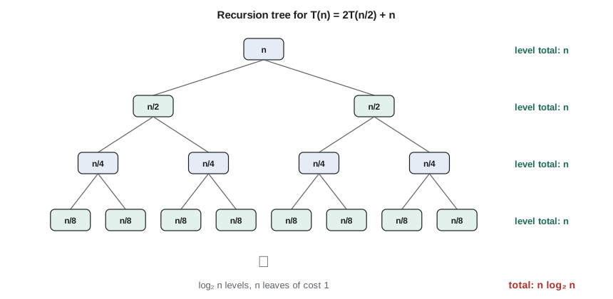
The number of leaves is a^(log_b n), which equals n^(log_b a). That quantity, the leaf count, is the benchmark the master theorem compares f(n) against. If f(n) grows more slowly than the leaf count, the leaves dominate. If they match, every level contributes equally. If f(n) grows faster, and the combine cost at each level shrinks by a constant factor as you go down, the root dominates.
The master theorem
Let c* = log_b a, the critical exponent. The master theorem states three cases. Case 1: if f(n) = O(n^(c* − ε)) for some ε > 0, then T(n) = Θ(n^c*). Case 2: if f(n) = Θ(n^c* · logᵏ n) for some k ≥ 0, then T(n) = Θ(n^c* · logᵏ⁺¹ n). Case 3: if f(n) = Ω(n^(c* + ε)) for some ε > 0, and a f(n/b) ≤ c f(n) for some c < 1 and large n (the regularity condition), then T(n) = Θ(f(n)).
| Algorithm | Recurrence | c* = log_b a | Case | Running time |
|---|---|---|---|---|
| Binary search | T(n) = T(n/2) + 1 | 0 | 2 (k = 0) | Θ(log n) |
| Merge sort | T(n) = 2T(n/2) + n | 1 | 2 (k = 0) | Θ(n log n) |
| Naive split multiplication | T(n) = 4T(n/2) + n | 2 | 1 | Θ(n²) |
| Karatsuba | T(n) = 3T(n/2) + n | about 1.585 | 1 | Θ(n^1.585) |
| Strassen matrix product | T(n) = 7T(n/2) + n² | about 2.807 | 1 | Θ(n^2.807) |
| Closest pair | T(n) = 2T(n/2) + n | 1 | 2 (k = 0) | Θ(n log n) |
| A heavy combine | T(n) = 2T(n/2) + n² | 1 | 3 | Θ(n²) |
The theorem does not cover everything. Recurrences with uneven splits, such as T(n) = T(n/3) + T(2n/3) + n, or with a subtraction rather than a division, such as T(n) = T(n − 1) + n, fall outside it; the recursion tree or the substitution method, guessing the answer and proving it by induction, handles those. The recursion tree for T(n/3) + T(2n/3) + n has levels costing n until the shorter branches run out, and its longest path has log_{3/2} n levels, so the answer is Θ(n log n).
Counting inversions
Dana's clock-drift check needs a measure of how out of order a node's records are when listed in the server's arrival order instead of the node's own timestamp order. The natural measure is the number of inversions: pairs i < j where a[i] > a[j]. Zero inversions means perfectly sorted; n(n − 1)/2 means perfectly reversed. Checking every pair takes Θ(n²) time, too slow for a year of records from a misbehaving node, about two million entries.
The divide-and-conquer algorithm piggybacks on merge sort. Split the list into halves, count the inversions within each half recursively while sorting it, and count the split inversions, pairs with one element in each half, during the merge. When the merge takes an element from the right half while k elements remain in the left half, that element is smaller than all k of them, which adds exactly k split inversions. The combine step stays linear, so the whole algorithm is Θ(n log n).
# Count inversions with merge sort, checked against the quadratic definition
def sort_count(a):
    if len(a) <= 1:
        return a, 0
    m = len(a) // 2
    left, x = sort_count(a[:m])
    right, y = sort_count(a[m:])
    merged, i, j, split = [], 0, 0, 0
    while i < len(left) and j < len(right):
        if left[i] <= right[j]:
            merged.append(left[i]); i += 1
        else:
            merged.append(right[j]); j += 1
            split += len(left) - i          # right[j] jumps over every remaining left item
    merged += left[i:] + right[j:]
    return merged, x + y + split

def slow(a):
    return sum(1 for i in range(len(a)) for j in range(i + 1, len(a)) if a[i] > a[j])

# node timestamps (seconds) in the order the server received them
arrivals = [3, 7, 1, 9, 12, 4, 15, 18, 16, 20, 22, 21]
print("fast:", sort_count(arrivals)[1], " slow:", slow(arrivals))

seed, data = 7, []
for _ in range(2000):
    seed = (1103515245 * seed + 12345) % 2**31
    data.append(seed % 10000)
print("2000 random values, fast == slow:", sort_count(data)[1] == slow(data))fast: 7 slow: 7 2000 random values, fast == slow: True
The same counting idea measures how similar two rankings are, the Kendall tau distance, which shows up in comparing the busiest-road rankings produced by two traffic models. It is also how recommendation systems compare one user's preferences with another's.
The closest pair of points
The planning group has the coordinates of all deployed counters projected onto a flat map in metres and wants the pair that is closest together. Checking all pairs costs Θ(n²), fine for 400 counters but not for the provincial dataset of 60,000 permanent and temporary count stations that a municipal client has asked Northway to clean. The divide-and-conquer algorithm runs in Θ(n log n).
Sort the points by x-coordinate. Split them with a vertical line into a left half and a right half, and find the closest pair in each half recursively; let δ be the smaller of the two distances. The closest pair overall is either one of those two or a pair that crosses the line. A crossing pair closer than δ must have both points within δ of the line, in a vertical strip of width 2δ. The surprising fact that makes the algorithm work is that, if the strip's points are sorted by y-coordinate, each point needs to be compared only with the next seven points in that order, because any square of side δ on one side of the line can contain at most four points that are all at least δ apart.
If the y-sorted order is maintained during the recursion, as merge sort does, the strip check is linear and the recurrence is T(n) = 2T(n/2) + Θ(n) = Θ(n log n). Implementations that re-sort the strip by y at every level take Θ(n log² n), which is still far better than quadratic and often fast enough.
Worked problem
Applying the master theorem
Solve T(n) = 4T(n/2) + n², T(n) = 9T(n/3) + n, and T(n) = 2T(n/4) + n.
Show solution
- First: a = 4, b = 2, c* = log₂ 4 = 2, and f(n) = n² = Θ(n² log⁰ n), so case 2 with k = 0 gives Θ(n² log n).
- Second: a = 9, b = 3, c* = log₃ 9 = 2, and f(n) = n = O(n^(2 − 1)), so case 1 gives Θ(n²).
- Third: a = 2, b = 4, c* = log₄ 2 = 0.5, and f(n) = n = Ω(n^(0.5 + 0.5)).
- Check regularity: a f(n/b) = 2(n/4) = n/2 ≤ (1/2) f(n), so case 3 gives Θ(n).
Answer: The comparison is always between f(n) and n^(log_b a). Computing the critical exponent first, before looking at f(n), avoids most mistakes.
Multiplying large integers
The firmware signing service at Northway verifies RSA signatures on every update package, and each verification multiplies numbers about 2,048 bits long. The schoolbook method multiplies every digit of one number by every digit of the other, Θ(n²) digit operations for n-digit numbers. Splitting each number into high and low halves, x = x₁·Bᵐ + x₀ and y = y₁·Bᵐ + y₀, gives four half-size products, and T(n) = 4T(n/2) + Θ(n) is still Θ(n²). Splitting alone gains nothing.
Karatsuba's insight in 1960 was that three multiplications suffice. Compute z₂ = x₁y₁ and z₀ = x₀y₀ as before, then compute (x₁ + x₀)(y₁ + y₀), which equals z₂ + z₁ + z₀ where z₁ = x₁y₀ + x₀y₁ is the middle term needed. Subtracting gives z₁ without a fourth product. The recurrence becomes T(n) = 3T(n/2) + Θ(n), which case 1 solves as Θ(n^(log₂ 3)) ≈ Θ(n^1.585).
# Karatsuba multiplication on Python integers (base 2, split by bit length)
def karatsuba(x, y, counter):
    if x < 2**32 or y < 2**32:
        counter[0] += 1                     # one hardware-sized multiply
        return x * y
    m = max(x.bit_length(), y.bit_length()) // 2
    x1, x0 = x >> m, x & ((1 << m) - 1)
    y1, y0 = y >> m, y & ((1 << m) - 1)
    z2 = karatsuba(x1, y1, counter)
    z0 = karatsuba(x0, y0, counter)
    z1 = karatsuba(x1 + x0, y1 + y0, counter) - z2 - z0
    return (z2 << (2 * m)) + (z1 << m) + z0

seed = 12345
def rand_bits(bits):
    global seed
    v = 0
    for _ in range(bits // 31 + 1):
        seed = (1103515245 * seed + 12345) % 2**31
        v = (v << 31) | seed
    return v >> (v.bit_length() - bits)

for bits in (512, 1024, 2048, 4096):
    a, b = rand_bits(bits), rand_bits(bits)
    c = [0]
    ok = karatsuba(a, b, c) == a * b
    school = (bits // 32) ** 2
print(f"{bits:5d} bits: correct={ok} base multiplies {c[0]:6d} schoolbook {school:6d}")512 bits: correct=True base multiplies 115 schoolbook 256 1024 bits: correct=True base multiplies 365 schoolbook 1024 2048 bits: correct=True base multiplies 1077 schoolbook 4096 4096 bits: correct=True base multiplies 3279 schoolbook 16384
In practice the base case matters. Below a few dozen machine words the schoolbook method's small constant wins, so libraries switch to Karatsuba only above a threshold and to even faster methods, Toom-Cook and then transforms based on the fast Fourier transform, for very large numbers. The same pattern, splitting into fewer subproblems by computing clever combinations, gives Strassen's matrix multiplication with seven half-size products instead of eight.
The fast Fourier transform, briefly
The most influential divide-and-conquer algorithm in engineering is the fast Fourier transform, which you met in ELE-250 and CMP-272. Evaluating a polynomial of degree n − 1 at the n complex roots of unity naively takes Θ(n²) operations. Splitting the polynomial into its even and odd coefficients gives two polynomials of half the degree, and the special symmetry of the roots of unity means each needs evaluating only at n/2 points. The recurrence T(n) = 2T(n/2) + Θ(n) gives Θ(n log n). Multiplying polynomials, and therefore very large integers, reduces to two transforms, a pointwise product and an inverse transform, which is why the fastest known integer multiplication algorithms are built on it.
Common mistakes
MistakeApplying the master theorem without computing log_b a first.
InsteadFind the critical exponent c* = log_b a, then compare f(n) with n^c*. Most errors come from comparing f(n) with the wrong benchmark.
MistakeSplitting a problem in half and expecting a speed-up without reducing the combine cost or the number of subproblems.
InsteadFour half-size products still give Θ(n²). The gain comes from fewer subproblems, as in Karatsuba, or a cheap combine.
MistakeUsing divide and conquer when subproblems overlap.
InsteadOverlapping subproblems make plain recursion exponential. Use dynamic programming to solve each subproblem once.
MistakeForgetting the regularity condition in case 3.
InsteadCheck that a f(n/b) ≤ c f(n) for some c < 1. Ordinary polynomial f(n) satisfies it, but unusual functions may not.
Summary and key terms
- Divide and conquer splits a problem into independent subproblems, solves them recursively and combines the answers.
- Running times satisfy T(n) = aT(n/b) + f(n); the recursion tree shows which levels dominate.
- The master theorem compares f(n) with n^(log_b a) and gives three cases: leaves dominate, all levels equal, or root dominates.
- Inversions are counted in Θ(n log n) by adding split inversions during the merge.
- The closest pair of points takes Θ(n log n) because each strip point needs only a constant number of comparisons.
- Karatsuba multiplies n-digit numbers in Θ(n^1.585) using three half-size products instead of four; the FFT gives Θ(n log n) evaluation.
- Divide and conquer
- A paradigm that solves independent smaller subproblems recursively and combines their solutions.
- Recurrence
- An equation that expresses a running time in terms of the running time on smaller inputs.
- Recursion tree
- A diagram of the cost at each level of a recursive algorithm, used to sum the total.
- Master theorem
- A rule that solves T(n) = aT(n/b) + f(n) by comparing f(n) with n^(log_b a).
- Inversion
- A pair of positions i < j with a[i] > a[j].
- Karatsuba multiplication
- A divide-and-conquer method that multiplies two numbers with three half-size products.
- Regularity condition
- The requirement in case 3 that a f(n/b) ≤ c f(n) for some constant c < 1.
Practice problems
Work each problem on paper first, then reveal the answer to check.
Solve T(n) = 8T(n/2) + n².
Show answer
c* = log₂ 8 = 3 and n² = O(n^(3 − 1)), so case 1 gives Θ(n³).
How many inversions does [4, 3, 2, 1] have?
Show answer
All 6 pairs are inverted: 4·3/2 = 6.
Why does the closest-pair strip check compare each point with only a few neighbours?
Show answer
Points on each side are at least δ apart, so only a constant number fit in the δ by 2δ box above any strip point.
Solve T(n) = T(n − 1) + n.
Show answer
The master theorem does not apply. Unrolling gives n + (n − 1) + … + 1 = n(n + 1)/2 = Θ(n²).
Lesson quiz · 5 questions
Score 60% or more to complete this lesson.
Create a free account to save your progress, take quizzes and earn a certificate.