
CMP-301 · Lesson 7 of 12 · 19 min
Shortest paths with negative edges and between all pairs
CMPUT-204 covers Dijkstra's algorithm, which finds shortest paths from one source when every edge weight is non-negative, in O((V + E) log V) time with a binary heap. Dijkstra's algorithm is greedy: it settles the closest unsettled vertex and never revisits it. That greedy choice is exactly what fails when some edges have negative weights, because a path that looks long now can become shorter later by passing through a negative edge. This lesson treats shortest paths as a dynamic programming problem, which handles negative edges and detects negative cycles, and then solves the all-pairs version, where every vertex is a source.
Negative edges sound artificial, but they appear naturally whenever an edge represents a gain rather than a cost. At Northway they come from clock synchronization. Each NS-4 node's real-time clock drifts by a few seconds a week, and the server knows bounds such as 'node 12's clock is at most 3 seconds ahead of node 7's' from overlapping traffic observations. Those bounds are difference constraints, and the solution is a shortest path problem whose edges can be negative. All-pairs shortest paths come from the field crew, who need travel times between every pair of depots and counter sites to plan maintenance routes.
Why Dijkstra fails with negative weights
Consider vertices s, a and b with edges s→a weight 2, s→b weight 5 and b→a weight −4. Dijkstra settles a first at distance 2, because it is the closest, and never changes it. But the path s→b→a has weight 5 − 4 = 1, which is shorter. Dijkstra's correctness proof relies on the fact that extending a path can never make it shorter, and a negative edge breaks that. Adding a constant to every weight to make them all non-negative does not fix the problem either, because it penalizes paths with more edges.
Negative cycles cause a deeper problem. If a cycle has negative total weight and is reachable from the source and can reach the destination, going around it again and again makes the path weight arbitrarily small, so no shortest path exists. Any algorithm that allows negative edges must detect negative cycles and report them. In the clock problem, a negative cycle means the constraints contradict each other, which signals a faulty node or a mistake in the observations.
The Bellman-Ford algorithm
Bellman-Ford is a dynamic program. Let d_k(v) be the weight of the shortest path from s to v that uses at most k edges. A shortest path with at most k edges either uses at most k − 1 edges, or ends with some edge u→v after a shortest path to u with at most k − 1 edges. If there is no negative cycle, a shortest path never repeats a vertex, so it has at most V − 1 edges, and d_{V−1}(v) is the true shortest distance.
In practice the algorithm keeps a single distance array and relaxes every edge V − 1 times. Relaxing edge u→v means replacing d(v) with d(u) + w(u, v) if that is smaller. After V − 1 rounds every shortest path has been found. One more round detects negative cycles: if any edge can still be relaxed, a negative cycle is reachable. The running time is O(VE), slower than Dijkstra but correct on every graph. An easy improvement stops early when a round changes nothing.
# Bellman-Ford with negative-cycle detection
def bellman_ford(nodes, edges, s):
    d = {v: float('inf') for v in nodes}; d[s] = 0
    pred = {v: None for v in nodes}
    for _ in range(len(nodes) - 1):
        changed = False
        for u, v, w in edges:
            if d[u] + w < d[v]:
                d[v] = d[u] + w; pred[v] = u; changed = True
        if not changed:
            break
    for u, v, w in edges:
        if d[u] + w < d[v]:
            return None, None          # a negative cycle is reachable
    return d, pred

nodes = ['s', 'a', 'b']
edges = [('s', 'a', 2), ('s', 'b', 5), ('b', 'a', -4)]
d, pred = bellman_ford(nodes, edges, 's')
print("distances:", d, " a is reached via", pred['a'])

bad = edges + [('a', 'b', 1)]          # b -> a -> b has weight -3
print("with cycle b->a->b:", bellman_ford(nodes, bad, 's'))distances: {'s': 0, 'a': 1, 'b': 5} a is reached via b
with cycle b->a->b: (None, None)Difference constraints and clock synchronization
A system of difference constraints is a set of inequalities of the form x_j − x_i ≤ c, where the x are unknowns and the c are constants. Dana's clock problem has exactly this form. Let x_i be the correction to apply to node i's clock. An observation that a vehicle passed node 7 and then node 12 at least 40 seconds later, given the road distance and speed limits, translates into a bound on the difference of their corrections. Dozens of such bounds connect the nodes along a corridor.
Build a constraint graph with a vertex for each unknown and, for each constraint x_j − x_i ≤ c, an edge from i to j with weight c. Add a source connected to every vertex with weight 0 and run Bellman-Ford from it. If there is a negative cycle, the constraints are infeasible. Otherwise the shortest distances x_i = d(i) satisfy every constraint, because the shortest-path property d(j) ≤ d(i) + w(i, j) is precisely x_j − x_i ≤ c. This reduction, from a system of inequalities to a shortest path problem, is a small example of the reductions that lesson 10 builds into a theory.
Worked problem
Finding consistent clock corrections
Four nodes have corrections x₁ to x₄ (seconds) with constraints x₂ − x₁ ≤ 3, x₃ − x₂ ≤ −2, x₄ − x₃ ≤ 4, x₁ − x₄ ≤ −1 and x₃ − x₁ ≤ 0. Find a feasible solution or show none exists.
Show solution
- Edges: 1→2 (3), 2→3 (−2), 3→4 (4), 4→1 (−1), 1→3 (0), plus a source 0 with weight-0 edges to all four.
- Check the cycle 1→2→3→4→1: 3 − 2 + 4 − 1 = 4, positive. Cycle 1→3→4→1: 0 + 4 − 1 = 3, positive. No negative cycle.
- Bellman-Ford from 0: d = 0 for all initially; relaxing 2→3 gives d(3) = −2; 3→4 keeps d(4) = 0 since −2 + 4 = 2 > 0; 4→1 gives d(1) = −1; 1→3 gives d(3) = min(−2, −1) = −2; 1→2 keeps d(2) = 0.
- Final: x₁ = −1, x₂ = 0, x₃ = −2, x₄ = 0.
- Check: x₂ − x₁ = 1 ≤ 3; x₃ − x₂ = −2 ≤ −2; x₄ − x₃ = 2 ≤ 4; x₁ − x₄ = −1 ≤ −1; x₃ − x₁ = −1 ≤ 0. All hold.
Answer: Adding any constant to every x keeps the constraints satisfied, so the server anchors the solution by fixing the correction of the node with a GPS time fix to zero.
All-pairs shortest paths
The field crew's planning tool needs the travel time between every pair of 25 depots and frequently visited sites. Running Dijkstra from each vertex costs O(V(V + E) log V), which is excellent for sparse road networks. When the graph is dense, or has negative edges, a dedicated all-pairs algorithm is simpler and often faster.
The Floyd-Warshall algorithm is another dynamic program, with a clever choice of subproblem. Number the vertices 1 to n. Let D_k(i, j) be the shortest path from i to j that uses only vertices 1 to k as intermediate stops. A shortest such path either does not use vertex k, giving D_{k−1}(i, j), or passes through k exactly once, giving the shortest path from i to k plus the shortest from k to j, both using only vertices 1 to k − 1.
The table can be updated in place, so the algorithm is three nested loops over k, i and j with a single n-by-n matrix, Θ(n³) time and Θ(n²) space. It handles negative edges, and a negative cycle shows up as a negative entry on the diagonal. Its simplicity makes it the usual choice for n up to a few hundred; for 25 vertices it does about 15,600 updates. Keeping a matrix of next hops alongside the distances lets the tool print the actual routes.
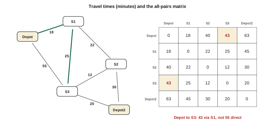
# Floyd-Warshall travel times (minutes) with route reconstruction
INF = float('inf')
names = ['Depot', 'S1', 'S2', 'S3', 'Depot2']
n = len(names)
roads = [(0, 1, 18), (0, 3, 55), (1, 2, 22), (1, 3, 25), (2, 4, 30),
         (3, 4, 20), (2, 3, 12)]
D = [[0 if i == j else INF for j in range(n)] for i in range(n)]
nxt = [[j if i == j else None for j in range(n)] for i in range(n)]
for i, j, w in roads:
    D[i][j] = D[j][i] = w; nxt[i][j] = j; nxt[j][i] = i

for k in range(n):
    for i in range(n):
        for j in range(n):
            if D[i][k] + D[k][j] < D[i][j]:
                D[i][j] = D[i][k] + D[k][j]; nxt[i][j] = nxt[i][k]

def route(i, j):
    path = [i]
    while i != j:
        i = nxt[i][j]; path.append(i)
    return " -> ".join(names[p] for p in path)

print("        " + " ".join(f"{m:>7s}" for m in names))
for i in range(n):
    print(f"{names[i]:7s} " + " ".join(f"{D[i][j]:7.0f}" for j in range(n)))
print("Depot to S3:", route(0, 3), f"({D[0][3]} min)")Depot S1 S2 S3 Depot2 Depot 0 18 40 43 63 S1 18 0 22 25 45 S2 40 22 0 12 30 S3 43 25 12 0 20 Depot2 63 45 30 20 0 Depot to S3: Depot -> S1 -> S3 (43 min)
Johnson's algorithm
For sparse graphs with negative edges, Johnson's algorithm combines the two approaches. It runs Bellman-Ford once from an added source to compute a potential h(v) for every vertex, then reweights each edge as w'(u, v) = w(u, v) + h(u) − h(v). The shortest-path property guarantees that every reweighted edge is non-negative, and every path between two vertices changes weight by the same amount h(start) − h(end), so shortest paths are unchanged. Dijkstra can then run from every vertex. The total is O(VE + V(V + E) log V), better than Floyd-Warshall when E is much smaller than V².
Choosing an algorithm
| Situation | Algorithm | Running time |
|---|---|---|
| One source, non-negative weights | Dijkstra with a binary heap | O((V + E) log V) |
| One source, negative weights possible | Bellman-Ford | O(VE) |
| One source, DAG | Topological order (lesson 5) | O(V + E) |
| All pairs, dense or small graph | Floyd-Warshall | Θ(V³) |
| All pairs, sparse, non-negative | Dijkstra from every vertex | O(V(V + E) log V) |
| All pairs, sparse, negative weights | Johnson | O(VE + V(V + E) log V) |
| Unweighted | Breadth-first search | O(V + E) |
Routing protocols on the internet use both families. Distance-vector protocols such as RIP are distributed versions of Bellman-Ford, in which each router repeatedly tells its neighbours its current distances; link-state protocols such as OSPF flood the topology to every router, which then runs Dijkstra locally. CMP-330 covers both. The slow convergence of distance-vector routing after a link fails, the count-to-infinity problem, is a direct consequence of Bellman-Ford's iterative relaxation.
Common mistakes
MistakeRunning Dijkstra on a graph with negative edges.
InsteadDijkstra's greedy settling assumes extending a path never shortens it. Use Bellman-Ford, or Johnson's reweighting, when weights can be negative.
MistakeAdding a constant to every edge to remove negative weights.
InsteadThat penalizes paths with more edges and changes which path is shortest. Johnson's potentials reweight without changing shortest paths.
MistakeForgetting the extra round of Bellman-Ford.
InsteadAfter V − 1 rounds, one more pass that still finds an improvement proves a reachable negative cycle.
MistakeOrdering the Floyd-Warshall loops as i, j, k.
InsteadThe intermediate-vertex index k must be the outermost loop so that D_{k−1} is complete before D_k is computed.
Summary and key terms
- Dijkstra's greedy choice fails when edges can have negative weights.
- Bellman-Ford relaxes every edge V − 1 times, runs in O(VE) and detects negative cycles with one extra pass.
- Difference constraints x_j − x_i ≤ c reduce to shortest paths; a negative cycle means the constraints are infeasible.
- Floyd-Warshall solves all pairs in Θ(V³) by allowing one more intermediate vertex at each step.
- Johnson's algorithm reweights edges with Bellman-Ford potentials so that Dijkstra can run from every vertex.
- Distance-vector routing is distributed Bellman-Ford; link-state routing runs Dijkstra at each router.
- Negative cycle
- A cycle whose edge weights sum to less than zero, which makes shortest paths undefined.
- Relaxation
- Improving a distance estimate d(v) using d(u) + w(u, v) for an edge from u to v.
- Bellman-Ford algorithm
- A single-source shortest path algorithm that allows negative weights and detects negative cycles.
- Difference constraint
- An inequality of the form x_j − x_i ≤ c between two unknowns.
- Floyd-Warshall algorithm
- A Θ(V³) dynamic program that computes shortest paths between all pairs of vertices.
- Johnson's algorithm
- All-pairs shortest paths for sparse graphs, reweighting edges so Dijkstra can be used.
- Potential
- A value h(v) per vertex used to reweight edges without changing shortest paths.
Practice problems
Work each problem on paper first, then reveal the answer to check.
How many relaxation rounds does Bellman-Ford need on a graph with 50 vertices, and what does round 50 show?
Show answer
49 rounds find all shortest paths; any improvement in round 50 proves a reachable negative cycle.
Translate x₃ − x₅ ≤ −7 into a constraint-graph edge.
Show answer
An edge from vertex 5 to vertex 3 with weight −7.
How many inner updates does Floyd-Warshall perform for 200 vertices?
Show answer
200³ = 8,000,000 updates.
Why must a shortest path have at most V − 1 edges when there are no negative cycles?
Show answer
Repeating a vertex creates a cycle of non-negative weight, which can be removed without lengthening the path, so some shortest path visits each vertex at most once.
Lesson quiz · 5 questions
Score 60% or more to complete this lesson.
Create a free account to save your progress, take quizzes and earn a certificate.