Dynamic programming II: edit distance, alignment, trees and DAGs

Lesson 4 built dynamic programs over a list of items and over pairs of prefixes. This lesson extends the method in three directions. Edit distance and sequence alignment generalize the longest common subsequence with costs for each kind of change, and show how to cut the memory of a two-dimensional table from quadratic to linear. Dynamic programming on directed acyclic graphs reveals that every dynamic program is secretly a shortest or longest path problem on the graph of its subproblems. Dynamic programming on trees solves problems that are hard on general graphs, such as choosing the fewest relays to cover a network, in linear time when the network is a tree.

Northway brings all three. The support team wants a tolerant way to match device serial numbers typed by field technicians, who routinely swap or mistype characters. The data pipeline that turns raw counts into reports is a set of dependent jobs whose critical path decides when the morning reports are ready. And in rural deployments, nodes relay each other's data along a tree-shaped mesh, where Maren needs to decide which nodes get the larger battery that lets them act as relays.

Edit distance

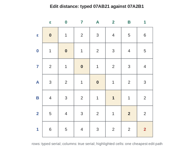
The edit distance between two strings is the smallest number of single-character insertions, deletions and substitutions that turns one into the other. It is also called the Levenshtein distance, after Vladimir Levenshtein, who defined it in 1965. A technician typing serial NS4-07A2B1 as NS4-07AB21 has made an error that is two substitutions, or a deletion and an insertion, away from the truth, while every other serial in the database is much further away.

Let D(i, j) be the edit distance between the first i characters of x and the first j characters of y. The last characters can be matched, at cost 0 if equal and 1 otherwise; or the last character of x can be deleted; or the last character of y can be inserted. The base cases say that turning a prefix into the empty string costs its length.

The table has (m + 1)(n + 1) entries filled row by row in constant time each, so the algorithm runs in Θ(mn) time. The bracket [x_i ≠ y_j] is 1 if the characters differ and 0 otherwise. Comparing a typed serial against 400 known serials of about ten characters takes about 40,000 table entries, instantaneous on any server.

# Edit distance with traceback, used to suggest the intended serial number
def edit(x, y):
    m, n = len(x), len(y)
    D = [[0] * (n + 1) for _ in range(m + 1)]
    for i in range(m + 1): D[i][0] = i
    for j in range(n + 1): D[0][j] = j
    for i in range(1, m + 1):
        for j in range(1, n + 1):
            D[i][j] = min(D[i - 1][j - 1] + (x[i - 1] != y[j - 1]),
                          D[i - 1][j] + 1, D[i][j - 1] + 1)
    ops, i, j = [], m, n
    while i or j:
        if i and j and D[i][j] == D[i - 1][j - 1] + (x[i - 1] != y[j - 1]):
            if x[i - 1] != y[j - 1]:
                ops.append(f"sub {x[i-1]}->{y[j-1]}")
            i -= 1; j -= 1
        elif i and D[i][j] == D[i - 1][j] + 1:
            ops.append(f"del {x[i-1]}"); i -= 1
        else:
            ops.append(f"ins {y[j-1]}"); j -= 1
    return D[m][n], ops[::-1]

known = ['NS4-07A2B1', 'NS4-07A2B7', 'NS4-17C9D4', 'NS4-03F1E8', 'NS4-07B2A1']
typed = 'NS4-07AB21'
ranked = sorted((edit(typed, k)[0], k) for k in known)
for d, k in ranked:
    print(f"{k}  distance {d}")
print("edits to best match:", edit(typed, ranked[0][1])[1])

NS4-07A2B1  distance 2
NS4-07B2A1  distance 2
NS4-07A2B7  distance 3
NS4-03F1E8  distance 5
NS4-17C9D4  distance 5
edits to best match: ['sub B->2', 'sub 2->B']

Two serials tie at distance 2, NS4-07A2B1 and NS4-07B2A1, which is itself useful information: the support tool shows both and asks the technician to read the label again rather than guessing. A variant called the Damerau-Levenshtein distance also allows swapping two adjacent characters at cost 1, which matches the most common typing error better and would rank NS4-07A2B1 first at distance 1.

Sequence alignment with general costs

Edit distance charges 1 for every operation. Sequence alignment allows any costs: a gap penalty δ for inserting or deleting, and a mismatch cost α(a, b) for aligning character a with character b. The recurrence keeps the same shape, with the constants replaced by the costs. Alignment with biologically chosen costs is how DNA and protein sequences are compared, and the algorithm, published by Needleman and Wunsch in 1970, is one of the most heavily used dynamic programs in science.

Costs can encode domain knowledge. For serial numbers, Jonah sets α(0, O) and α(1, I) to 0.3, because those characters look alike on a weathered label, and every other mismatch to 1. For comparing sequences of vehicle classes from two counters on the same road, which should agree except for vehicles one missed, a mismatch between a car and a light truck is cheap and between a car and a bus is expensive.

Linear space

An alignment table for two sequences of length 100,000, such as a day of per-vehicle records from two counters at the same site, has ten billion entries. The time is acceptable, but the memory is not. If only the distance is needed, two rows suffice, because each row depends only on the one above, and the space falls to Θ(n). Recovering the alignment itself is harder, because the traceback needs the whole table.

Hirschberg's algorithm, from 1975, recovers the full alignment in linear space and still Θ(mn) time by combining dynamic programming with divide and conquer. It runs the two-row computation forward from the start over the first half of x, and backward from the end over the second half, and finds the column where the optimal path crosses the middle row by adding the two halves' costs. It then recurses on the two smaller problems on either side of that crossing point. The total work is at most twice the single-pass work, because the subproblems shrink geometrically.

Every dynamic program is a path in a DAG

Draw each subproblem as a vertex and draw an edge from each subproblem to every subproblem that uses it, weighted by the cost that the recurrence adds. Because each subproblem depends only on smaller ones, the graph has no cycles: it is a directed acyclic graph, a DAG. Filling the table in a valid order is processing the vertices in topological order, and the recurrence's min or max is the relaxation step of a shortest or longest path algorithm. Edit distance, for example, is the shortest path from the top-left corner to the bottom-right corner of the grid graph whose edges cost 0 or 1.

Shortest and longest paths in a DAG take Θ(V + E) time: sort the vertices topologically, then relax each vertex's outgoing edges once in that order. Longest paths are worth singling out. On a general graph the longest simple path is an NP-hard problem, but on a DAG it is easy, and it is the basis of the critical path method used to schedule projects, which CON-310 applies to construction. Northway's nightly data pipeline is a DAG of jobs, and the longest path through it decides when the morning reports are ready.

# Critical path of the nightly pipeline: longest path in a DAG
from collections import defaultdict, deque

duration = {'ingest': 20, 'dedupe': 15, 'classify': 40, 'weather': 10,
            'quality': 25, 'aggregate': 30, 'reports': 15}
needs = {'dedupe': ['ingest'], 'classify': ['dedupe'], 'weather': ['ingest'],
         'quality': ['dedupe', 'weather'], 'aggregate': ['classify', 'quality'],
         'reports': ['aggregate']}

succ, indeg = defaultdict(list), {j: 0 for j in duration}
for job, pre in needs.items():
    for p in pre:
        succ[p].append(job); indeg[job] += 1

order, q = [], deque(j for j in duration if indeg[j] == 0)
while q:
    j = q.popleft(); order.append(j)
    for k in succ[j]:
        indeg[k] -= 1
        if indeg[k] == 0:
            q.append(k)

finish, prev = {}, {}
for j in order:
    start = max((finish[p] for p in needs.get(j, [])), default=0)
    prev[j] = max(needs.get(j, []), key=lambda p: finish[p], default=None)
    finish[j] = start + duration[j]

path, j = [], 'reports'
while j:
    path.append(j); j = prev[j]
print("topological order:", order)
print("critical path:", " -> ".join(reversed(path)), f"({finish['reports']} min)")

topological order: ['ingest', 'dedupe', 'weather', 'classify', 'quality', 'aggregate', 'reports']
critical path: ingest -> dedupe -> classify -> aggregate -> reports (120 min)

Starting at 01:00, the reports are ready at 03:00. Shortening the weather join or the quality checks would not help, because they are not on the critical path; speeding up classification, the longest job on it, would. That observation alone saved Dana from optimizing the wrong job.

Dynamic programming on trees

Many problems that are hard on general graphs become easy on trees, because a tree has no cycles and every vertex separates the tree into independent subtrees below it. The usual pattern is to root the tree and compute, for each vertex, a small table of answers for the subtree below it, under each possible state of the vertex itself, combining the children's tables. A post-order traversal visits children before parents, so the whole computation takes linear time.

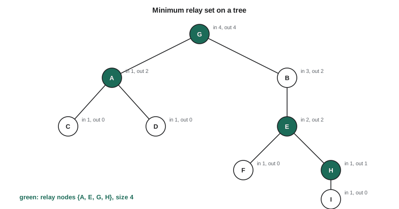
Maren's relay question is a vertex cover problem. In a rural deployment the nodes form a tree, and every link between two nodes needs at least one end equipped with the larger relay battery, so that the link stays up overnight. The batteries cost money, so she wants the smallest set of relay nodes covering every link. Lesson 11 shows that minimum vertex cover is NP-hard on general graphs. On a tree it is easy.

For each vertex u, compute two values: in(u), the smallest cover of u's subtree that includes u, and out(u), the smallest cover of u's subtree that excludes u. If u is in the cover, every edge to a child is already covered, so each child may be in or out, whichever is cheaper. If u is out, every edge to a child must be covered by the child, so every child must be in.

# Minimum vertex cover on a tree of relay nodes (post-order dynamic program)
links = [('G', 'A'), ('G', 'B'), ('A', 'C'), ('A', 'D'), ('B', 'E'),
         ('E', 'F'), ('E', 'H'), ('H', 'I')]
children = {}
for p, c in links:
    children.setdefault(p, []).append(c)

def solve(u):
    take, skip = 1, 0
    take_set, skip_set = [u], []
    for c in children.get(u, []):
        ci, co, si, so = solve(c)
        if ci <= co:
            take += ci; take_set += si
        else:
            take += co; take_set += so
        skip += ci; skip_set += si
    return take, skip, take_set, skip_set

ti, to, si, so = solve('G')
best = si if ti <= to else so
print("in(G) =", ti, " out(G) =", to)
print("relay nodes:", sorted(best), "count", len(best))
print("every link covered:", all(p in best or c in best for p, c in links))

in(G) = 4  out(G) = 4
relay nodes: ['A', 'E', 'G', 'H'] count 4
every link covered: True

The same pattern solves maximum-weight independent sets on trees, optimal placement of facilities along a tree, and the evaluation of expressions represented as trees. Graphs that are 'almost trees', with small treewidth, admit similar algorithms that are exponential only in the treewidth, an idea lesson 12 returns to when it discusses parameterized algorithms.