Network flow and bipartite matching

Many problems are about moving something through a network with limited capacity: data through links, vehicles through roads, current through wires, or people into jobs. The maximum flow problem captures them all, and it has two remarkable properties. It can be solved efficiently by a simple augmenting-path idea, and its answer always equals the capacity of the narrowest bottleneck, a fact called the max-flow min-cut theorem. Better still, an astonishing range of problems that do not look like flow at all, from assigning technicians to sites to deciding which counters to keep in a budget, can be reduced to it. This lesson develops the Ford-Fulkerson method, proves the max-flow min-cut theorem and uses flow to solve bipartite matching.

Northway's flow problem is literal. In the Kingston region, about 60 counters send their nightly data over low-power radio to a handful of solar gateways, which forward it over cellular links to the server. Each radio link and each cellular link can carry only so many megabytes in the overnight window. Dana wants to know how much data the network can move in that window and where the bottleneck is, because a new municipal contract will triple the number of counters.

Flow networks

A flow network is a directed graph with a source s, a sink t and a non-negative capacity c(e) on each edge. A flow assigns a value f(e) to each edge satisfying two rules. The capacity constraint says 0 ≤ f(e) ≤ c(e). Conservation says that at every vertex other than s and t, the flow in equals the flow out. The value of the flow is the net amount leaving s, which by conservation equals the net amount entering t. The maximum flow problem asks for a flow of largest value.

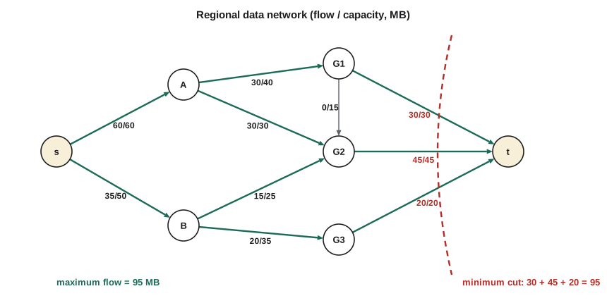
For Northway's network, the source is a super-source connected to every counter with capacity equal to that counter's nightly batch size, the sink is the server, and the other edges are radio and cellular links with their capacities. A maximum flow tells Dana how much data can arrive in the window; if it is less than the total of all batches, some data will wait until the next night.

Residual graphs and augmenting paths

The natural greedy idea, finding any path from s to t with spare capacity and pushing as much as possible along it, can get stuck at a flow that is not maximum, because an early path may use an edge in a way that blocks better choices. The fix is to allow later paths to undo earlier decisions. The residual graph G_f records, for each edge e from u to v with flow f(e), a forward edge with residual capacity c(e) − f(e), and a backward edge from v to u with residual capacity f(e). Pushing flow along a backward edge cancels flow that was sent earlier.

An augmenting path is a path from s to t in the residual graph. Its bottleneck is the smallest residual capacity along it. Augmenting adds the bottleneck to every forward edge on the path and subtracts it from every edge whose backward copy the path uses. The result is still a valid flow and its value has grown by the bottleneck.

The Ford-Fulkerson method, published in 1956, repeats this until no augmenting path exists. With integer capacities each augmentation increases the flow by at least 1, so the method terminates after at most |f*| augmentations, where |f*| is the maximum flow value. Each augmentation costs O(E) to find a path, giving O(E·|f*|) in total, which is pseudo-polynomial: a network whose capacities are a million can take a million augmentations if paths are chosen badly.

Edmonds-Karp

Choosing the shortest augmenting path, in number of edges, found by breadth-first search, removes the dependence on capacity values. Edmonds and Karp proved in 1972 that this rule needs at most O(VE) augmentations, giving O(VE²) total time regardless of the capacities. Faster algorithms exist, push-relabel methods run in O(V³) or better and recent theoretical results approach linear time, but Edmonds-Karp is simple, reliable and fast enough for networks of thousands of vertices.

# Edmonds-Karp maximum flow on the regional data network (capacities in MB)
from collections import deque, defaultdict

def max_flow(cap, s, t):
    flow = defaultdict(int)
    def residual(u, v):
        return cap.get((u, v), 0) - flow[(u, v)] + flow[(v, u)]
    nodes = {u for u, v in cap} | {v for u, v in cap}
    adj = defaultdict(set)
    for u, v in cap:
        adj[u].add(v); adj[v].add(u)
    total, paths = 0, 0
    while True:
        parent, q = {s: None}, deque([s])
        while q and t not in parent:
            u = q.popleft()
            for v in sorted(adj[u]):
                if v not in parent and residual(u, v) > 0:
                    parent[v] = u; q.append(v)
        if t not in parent:
            break
        path, v = [], t
        while parent[v] is not None:
            path.append((parent[v], v)); v = parent[v]
        b = min(residual(u, v) for u, v in path)
        for u, v in path:
            back = min(b, flow[(v, u)])           # cancel reverse flow first
            flow[(v, u)] -= back
            flow[(u, v)] += b - back
        total += b; paths += 1
    reach = set(parent)
    cut = [(u, v) for (u, v) in cap if u in reach and v not in reach]
    return total, paths, cut

cap = {('s', 'A'): 60, ('s', 'B'): 50, ('A', 'G1'): 40, ('A', 'G2'): 30,
       ('B', 'G2'): 25, ('B', 'G3'): 35, ('G1', 'G2'): 15, ('G1', 't'): 30,
       ('G2', 't'): 45, ('G3', 't'): 20}
value, n_paths, cut = max_flow(cap, 's', 't')
print("maximum flow:", value, "MB using", n_paths, "augmenting paths")
print("minimum cut edges:", sorted(cut), "capacity", sum(cap[e] for e in cut))

maximum flow: 95 MB using 4 augmenting paths
minimum cut edges: [('G1', 't'), ('G2', 't'), ('G3', 't')] capacity 95

Cuts and the max-flow min-cut theorem

An s-t cut divides the vertices into two sets, S containing s and T containing t. Its capacity is the total capacity of edges from S to T. Every unit of flow from s to t must cross from S to T somewhere, so the value of any flow is at most the capacity of any cut. This weak duality is easy. The max-flow min-cut theorem says the bound is tight: the maximum flow value equals the minimum cut capacity.

The proof comes straight from Ford-Fulkerson. When no augmenting path remains, let S be the set of vertices reachable from s in the residual graph and T the rest. Every edge from S to T must be saturated, or its residual capacity would make its far end reachable, and every edge from T to S must carry zero flow, or its backward residual edge would do the same. So the flow across the cut equals the cut's capacity, and since no flow can exceed any cut, this flow is maximum and this cut is minimum. The proof also gives an algorithm for the minimum cut: run max flow and collect the edges leaving the reachable set.

For Dana the cut is the actionable output. The flow value says how much data gets through; the cut says which links to upgrade. Upgrading a link that is not in a minimum cut does nothing, which is the flow-network version of the critical path lesson from lesson 5. In the example the minimum cut is the three links into the server, totalling 95 MB, so adding counters behind more gateways would not help until the cellular backhaul is upgraded.

Integrality

If all capacities are integers, Ford-Fulkerson only ever adds integer bottlenecks, so it finds a maximum flow in which every edge carries an integer amount. This integrality theorem is what makes flow such a powerful modelling tool: problems about indivisible things, people, jobs, time slots, can be modelled with integer capacities, solved as flows, and the answer read off as a valid integer assignment.

Bipartite matching

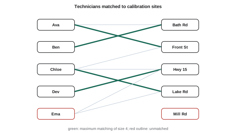
A bipartite graph has its vertices split into two sides, L and R, with every edge going between the sides. A matching is a set of edges no two of which share a vertex, and a maximum matching is one with as many edges as possible. Each spring Northway must recalibrate counters at sites around the region, and each technician is certified for certain counter models and lives within range of certain sites. Assigning each technician at most one site per day and each site at most one technician is a bipartite matching problem.

The reduction to flow is direct. Add a source connected to every technician with capacity 1, connect each technician to each site they can serve with capacity 1, and connect every site to a sink with capacity 1. An integer flow of value k picks k technician-site edges with no technician or site used twice, which is a matching of size k, and every matching gives a flow of the same value. So the maximum flow is the size of the maximum matching. Ford-Fulkerson runs in O(VE) here, since the flow value is at most V; the Hopcroft-Karp algorithm improves this to O(E√V).

# Maximum bipartite matching by augmenting paths (Kuhn's algorithm)
can_serve = {
    'Ava':   ['Bath Rd', 'Front St'],
    'Ben':   ['Bath Rd'],
    'Chloe': ['Front St', 'Hwy 15', 'Lake Rd'],
    'Dev':   ['Hwy 15'],
    'Ema':   ['Lake Rd', 'Hwy 15'],
}
sites = sorted({s for v in can_serve.values() for s in v} | {'Mill Rd'})
match = {}                       # site -> technician

def try_assign(tech, seen):
    for site in can_serve[tech]:
        if site in seen:
            continue
        seen.add(site)
        if site not in match or try_assign(match[site], seen):
            match[site] = tech
            return True
    return False

size = sum(try_assign(t, set()) for t in can_serve)
for site in sites:
    print(f"{site:9s} <- {match.get(site, '(unassigned)')}")
print("matching size:", size)

Bath Rd   <- Ben
Front St  <- Ava
Hwy 15    <- Dev
Lake Rd   <- Chloe
Mill Rd   <- (unassigned)
matching size: 4

Five technicians and five sites give a matching of only four on this day. The reason is simple once seen: between them, the five technicians can serve only four sites, because nobody certified lives near Mill Road, so at most four can be busy and one technician, here Ema, has no site. König's theorem, the bipartite analogue of max-flow min-cut, says the size of a maximum matching equals the size of a minimum vertex cover in a bipartite graph, so a small set of vertices that touch every edge certifies that no larger matching exists. Hall's theorem gives the condition for a perfect matching: every set of k technicians must collectively be able to serve at least k sites.

Other problems that reduce to flow

Flow models go far beyond moving data. Edge-disjoint paths, the number of link-independent routes between two gateways, equals the maximum flow with unit capacities, which measures how many links can fail before a gateway is cut off. Circulations with demands model supply and demand at many points at once. Project selection, choosing which counters to keep when each has a value and some depend on others, reduces to a minimum cut. Image segmentation in computer vision, separating foreground from background, is a minimum cut on a pixel grid. Airline crew scheduling and baseball elimination problems are other classic reductions. The skill is recognizing when a problem's constraints are capacities and its decisions are flows.