
CHE-470 · Lesson 12 of 12 · 22 min
Refinery planning and economics: the capstone
Theo's secondment ends with a capstone exercise. Sanjay has asked him to build a small version of the refinery's planning model, use it to choose next quarter's crude slate between a light crude and diluted bitumen, and then use the same tools to frame the two big decisions waiting on the refinery's management: whether to build the hydrocracker, and how to cut the refinery's carbon dioxide emissions. Roz will review his work, and he will present it to the refinery's leadership team before he returns to Kingfisher. Everything in the course feeds into this lesson: the assay data of lesson 2, the unit yields and limits of lessons 3 to 10, and the hydrogen and emissions balance of lesson 11.
How refineries make money
A refinery's gross margin is the value of its products minus the cost of its crude and other feeds. From that it must pay its operating costs: energy, catalysts and chemicals, labour, maintenance, and in many jurisdictions carbon costs. What is left must cover the return on the capital tied up in the plant. Refining is a high-volume, low-margin business. A margin of a few dollars a barrel on 120,000 barrels a day is a large sum, but small changes in prices or in the refinery's operations can swing it from profit to loss.
The industry's simplest margin indicator is the crack spread, the difference between the value of products and the cost of crude. The 3-2-1 crack spread assumes that three barrels of crude make two barrels of gasoline and one of diesel:
with all prices in dollars per barrel. Benchmark prices are quoted in US dollars, gasoline and diesel usually per gallon, so they must be converted at 42 US gallons per barrel. The code uses a crude price of 72 dollars per barrel, gasoline at 2.30 dollars per gallon and diesel at 2.55, and finds a 3-2-1 crack spread of about 28 dollars per barrel. The crack spread is a market indicator, not a refinery's actual margin, which depends on its crude slate, configuration, product mix and costs, but it moves with refinery profitability and is watched daily.
Linear programming for refinery planning
Every major refinery plans with a linear programming (LP) model. The model represents each unit by its yields per barrel of feed, its capacity and its quality constraints, and represents crude and product prices, blending specifications and logistics limits. It then finds the combination of crudes, unit operations and product blends that maximizes margin while respecting every constraint. Large refinery LPs have thousands of variables and constraints, and many use non-linear refinements solved by successive linear programming, but the principle is the same as in a two-variable problem.
Theo's simplified model has two crudes. Crude A is a light crude, giving 48 % gasoline, 34 % diesel and 10 % residue, with a margin of 11 dollars per barrel at current prices. Crude B is a dilbit-like heavy crude, giving 36 % gasoline, 30 % diesel and 28 % residue, with a margin of 14.50 dollars per barrel, because its discount more than pays for its poorer yields as long as the coker can convert the residue. There are three constraints: the crude unit can take at most 120,000 b/d in total, the coker can take at most 26,000 b/d of residue, as Theo found in lesson 6, and the diesel hydrotreater can take at most 40,000 b/d of diesel.
In a two-variable LP, the optimum always lies at a corner of the feasible region, where two constraint lines meet. The code finds every corner, checks which are feasible and evaluates the margin at each.
# Refinery planning: a small linear program solved by checking corner points, and the 3-2-1 crack spread
import itertools
# Crude A (light) and crude B (heavy dilbit-like); yields per barrel and margin per barrel (illustrative)
yields = {"A": {"gasoline": 0.48, "diesel": 0.34, "residue": 0.10}, "B": {"gasoline": 0.36, "diesel": 0.30, "residue": 0.28}}
margin = {"A": 11.0, "B": 14.5}     # dollars per barrel after crude price discount
cdu_max = 120000
coker_max = 26000   # residue the coker can take, b/d
diesel_hdt = 40000  # diesel hydrotreater limit, b/d
def feasible(a, b):
    return (a >= 0 and b >= 0 and a + b <= cdu_max + 1e-6 and
            yields["A"]["residue"] * a + yields["B"]["residue"] * b <= coker_max + 1e-6 and
            yields["A"]["diesel"] * a + yields["B"]["diesel"] * b <= diesel_hdt + 1e-6)
# constraint lines: a+b=cdu, ra*a+rb*b=coker, da*a+db*b=hdt, axes
lines = [(1, 1, cdu_max), (0.10, 0.28, coker_max), (0.34, 0.30, diesel_hdt), (1, 0, 0), (0, 1, 0)]
best = None
for (a1, b1, c1), (a2, b2, c2) in itertools.combinations(lines, 2):
    det = a1 * b2 - a2 * b1
    if abs(det) < 1e-12: continue
    a = (c1 * b2 - c2 * b1) / det + 0.0; b = (a1 * c2 - a2 * c1) / det + 0.0
    if feasible(a, b):
        val = margin["A"] * a + margin["B"] * b
        print(f"corner A {abs(a) if abs(a) < 0.5 else a:8.0f}  B {b:8.0f}  margin {val/1e6:5.3f} million/d")
        if best is None or val > best[0]: best = (val, a, b)
print(f"best: crude A {best[1]:.0f} b/d, crude B {best[2]:.0f} b/d, margin {best[0]/1e6:.3f} million dollars per day")
# 3-2-1 crack spread (dollars per barrel of crude): 3 crude -> 2 gasoline + 1 diesel
crude, gas, dsl = 72.0, 2.30 * 42, 2.55 * 42   # crude per bbl; product prices per gallon x 42
print(f"3-2-1 crack spread {(2*gas + dsl - 3*crude)/3:.2f} dollars per barrel")corner A 42222 B 77778 margin 1.592 million/d corner A 100000 B 20000 margin 1.390 million/d corner A 0 B 92857 margin 1.346 million/d corner A 117647 B 0 margin 1.294 million/d corner A 0 B 0 margin 0.000 million/d best: crude A 42222 b/d, crude B 77778 b/d, margin 1.592 million dollars per day 3-2-1 crack spread 28.10 dollars per barrel
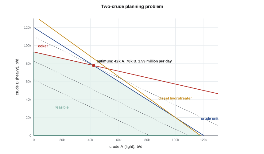
The best corner is about 42,000 b/d of crude A and 78,000 b/d of crude B, earning about 1.59 million dollars per day. At that point the crude unit is full and the coker is full; the diesel hydrotreater has some spare capacity, at about 37,700 b/d. Running all heavy crude would earn more per barrel but overload the coker, so the model fills the coker with as much heavy crude as it can take and makes up the rest of the crude unit with light crude.
Shadow prices
The most useful output of an LP is often not the plan itself but the shadow prices: the increase in margin from one more unit of each binding constraint. For the coker, adding one barrel per day of residue capacity lets the model swap light crude for heavy. Working through the two binding constraints, each extra barrel of coker capacity allows about 5.6 more barrels of crude B in place of crude A, worth \(5.6 \times 3.5 \approx 19\) dollars per day. For the crude unit, one more barrel of capacity, with the coker still full, is worth about 9 dollars per day. The diesel hydrotreater, not binding, has a shadow price of zero: more capacity there would earn nothing under these prices.
These numbers frame investment questions. A coker debottleneck that adds 2,000 b/d of residue capacity would be worth about 39,000 dollars per day, or about 14 million a year, before costs. That gives an upper bound on what the debottleneck could be worth paying for. Sanjay's real model shows similar results, which is why the planners keep returning to the coker drum cycle time Theo looked at in lesson 6.
| Constraint | Limit | At optimum | Binding? | Shadow price |
|---|---|---|---|---|
| Crude unit | 120,000 b/d | 120,000 b/d | Yes | about 9 dollars per b/d |
| Coker residue | 26,000 b/d | 26,000 b/d | Yes | about 19 dollars per b/d |
| Diesel hydrotreater | 40,000 b/d | about 37,700 b/d | No | zero |
From the LP to the real refinery
Real planning models add many refinements. Unit yields depend on feed quality, so crudes are represented by their assays, with each cut sent to the units it can feed. Product blending is modelled with octane, vapour pressure, sulfur and other specifications, using the blending rules of lesson 8. Hydrogen, fuel gas and steam balances link the units. Seasonal product specifications change the gasoline recipes. Inventory and logistics constraints, including pipeline schedules and tank capacity, limit what can be bought and sold in each period. Prices come from forward markets and the refinery's own contracts.
The monthly plan is then turned into a daily schedule by schedulers, who decide when each crude tank is run, when each product batch is blended and shipped, and how units respond to upsets. Advanced process control, in turn, holds each unit at the targets the plan sets. The planning, scheduling and control layers together make up the refinery's optimization chain. Each step relies on accurate data: the assays from lesson 2, unit tests that measure actual yields, and laboratory and analyzer measurements of product quality.
Evaluating the hydrocracker
The hydrocracker decision is a capital project. A 12,000 b/d hydrocracker, with its share of a new or expanded hydrogen plant, sulfur and utilities, is a large investment. Its benefit comes from upgrading gas oil that would otherwise go to the FCC, or be sold, into higher-value diesel and jet fuel with a volume gain of about 22 %, as in lesson 6. Its costs include hydrogen, energy, catalyst and maintenance, plus the carbon cost of the extra hydrogen. The evaluation compares the net present value of the project's cash flows under a range of price scenarios.
Theo runs the planning model with and without the hydrocracker under three scenarios: one with the diesel crack spread at its five-year average, one with diesel strong, and one in which diesel demand falls faster than expected. He also adds the hydrogen supply cost and carbon cost from lesson 11, which make a large difference: with a conventional SMR, the hydrocracker's hydrogen adds roughly 400 t/d of carbon dioxide, using the 8.7 t per tonne of hydrogen from lesson 11. The results show that the project is attractive in the base and strong-diesel cases but marginal if diesel demand falls, and that its value depends heavily on the cost and carbon intensity of the hydrogen supply.
Roz's advice is to present the decision as a set of trade-offs rather than a single answer. Leadership will want to know which assumptions drive the result, how robust it is to prices, and what alternatives exist, such as a smaller, cheaper FCC feed hydrotreater, which would improve FCC yields with less hydrogen, or a phased approach that builds the low-carbon hydrogen supply first.
The emissions roadmap and the energy transition
Theo's emissions roadmap from lesson 11 goes into the same model. Each option, such as furnace efficiency upgrades, SMR capture, co-processing renewable feed or buying lower-carbon ethanol, has a capital cost, an operating cost and a carbon dioxide reduction, and some also change the products' carbon intensity and earn compliance credits under the Clean Fuel Regulations. The model ranks them by cost per tonne of carbon dioxide avoided and shows how the ranking changes with carbon prices and credit values. Energy efficiency comes first, as expected; capture at the SMR comes next if a storage route is available; and renewable co-processing depends on feedstock prices.
The longer view is uncertain. Demand for gasoline in North America has flattened as vehicles become more efficient and electric vehicles gain share, while demand for diesel, jet fuel and petrochemicals has held up better. Refineries are responding in different ways: some by closing or converting to renewable fuels, some by integrating more closely with petrochemicals as in lesson 10, and some by investing to become the lowest-cost, lowest-emission supplier in their region so that they are among the last to close. Theo's report does not try to predict which path the St. Clair refinery will take, but sets out the questions each investment must answer.
Theo's presentation
Theo presents to the leadership team in the refinery's main conference room. He shows the planning model, the shadow price on the coker, the hydrocracker scenarios and the emissions roadmap, and he finishes with the idea Nadia raised in lesson 10: that Kingfisher's ethanol could be supplied to the refinery for blending today and, if markets develop, dehydrated to bio-ethylene for a neighbouring chemical plant. Bea asks how the coker drum cycle could be shortened safely; Sanjay asks for the hydrocracker case to be rerun with a range of hydrogen prices; and the refinery manager asks Theo to stay in touch when he returns to Kingfisher, since the two companies may have more to do together.
Back at Kingfisher, Ingrid asks what he learned. Theo's answer is that a refinery is one large, connected system, where every unit's limits, every crude's assay and every product's specification meet in a single optimization, and where the next decade's decisions depend as much on hydrogen and carbon as on crude and gasoline.
Worked problem
Shadow price of the coker
In Theo's model, with the crude unit full and the coker full, show that one more barrel per day of coker capacity is worth about 19 dollars per day.
Show solution
- With \(x_{A} + x_{B} = 120\,000\) and \(0.10\,x_{A} + 0.28\,x_{B} = 26\,000\), substitute: \(12\,000 + 0.18\,x_{B} = 26\,000\).
- One more barrel of coker capacity raises \(x_{B}\) by \(1/0.18 = 5.56\) b/d and lowers \(x_{A}\) by the same amount.
- Margin change: \(5.56 \times (14.5 - 11) = 19.4\) dollars per day.
Answer: About 19 dollars per day per barrel of coker capacity.
Common mistakes
MistakeTreating the crack spread as the refinery's margin.
InsteadIt is a market indicator; actual margin depends on crude, configuration and costs.
MistakeReading only the optimal plan from an LP.
InsteadShadow prices show which constraints are worth relieving.
MistakeEvaluating a project at one set of prices.
InsteadRun scenarios; show which assumptions drive the result.
MistakeLeaving hydrogen and carbon costs out of a conversion project.
InsteadThey can decide whether a hydrocracker pays.
Summary and key terms
- Refinery margin is product value minus crude cost; the 3-2-1 crack spread is a market indicator of it.
- Linear programming chooses crudes, unit operations and blends to maximize margin within constraints.
- Shadow prices show the value of relieving each binding constraint and guide debottlenecking.
- Capital projects are judged on scenarios, including hydrogen and carbon costs.
- Emissions options are ranked by cost per tonne avoided within the same planning framework.
- Crack spread
- The difference between the value of refined products and the cost of crude, per barrel.
- Linear programming
- An optimization method for linear objectives and constraints, used for refinery planning.
- Binding constraint
- A constraint that is at its limit in the optimal solution.
- Shadow price
- The increase in the objective per unit increase in a binding constraint.
- Net present value
- The discounted sum of a project's future cash flows minus its investment.
- Debottlenecking
- Raising the capacity of the constraint that limits a plant.
Practice problems
Work each problem on paper first, then reveal the answer to check.
What does the 3-2-1 crack spread assume?
Show answer
Three barrels of crude make two of gasoline and one of diesel.
Why does the LP optimum lie at a corner?
Show answer
The objective is linear, so it is maximized at a vertex of the feasible region.
What is the shadow price of a non-binding constraint?
Show answer
Zero.
Why does the model not run all heavy crude?
Show answer
The coker cannot take all the residue.
Name two costs that must be in a hydrocracker evaluation.
Show answer
Hydrogen supply and carbon costs, along with energy, catalyst and capital.
How are emissions options ranked?
Show answer
By cost per tonne of carbon dioxide avoided.
Lesson quiz · 5 questions
Score 60% or more to complete this lesson.
Create a free account to save your progress, take quizzes and earn a certificate.