Population growth and regulation

A population is a group of individuals of one species living in the same area, and its size changes for only four reasons: births add individuals, deaths remove them, immigration brings them in and emigration takes them out. Everything that happens to a population, from the explosive spread of zebra mussels through the Great Lakes to the slow recovery of whooping cranes, is a matter of these four processes. BIOL-108 introduced exponential and logistic growth in outline. This lesson develops them properly: how growth rates are measured, why growth eventually slows, how the timing of density dependence can make populations cycle or behave chaotically, how chance events threaten small populations, and what regulates real populations in nature.

Exponential growth

If every individual has the same average chance of giving birth and of dying, and these chances do not change as the population grows, the population grows by a constant proportion each unit of time. For populations that breed continuously, the rate of change is proportional to population size:

Here \( r \) is the intrinsic rate of increase: the per capita birth rate minus the per capita death rate when resources are unlimited. For species that breed once a year in a pulse, such as many birds and fish, growth is better described in discrete steps with the finite rate of increase \( \lambda \), the ratio of population size in one year to the year before:

When \( r > 0 \) (or \( \lambda > 1 \)) the population grows; when \( r < 0 \) (\( \lambda < 1 \)) it shrinks. A useful rule of thumb is that the doubling time is about 0.693 divided by \( r \).

import math
for name, r in [("bacteria (per hour)", 1.4), ("house mice (per week)", 0.05),
                ("white-tailed deer (per year)", 0.35), ("grizzly bear (per year)", 0.04)]:
    td = math.log(2) / r
    print(f"{name:30s} r = {r:5.2f}  lambda = {math.exp(r):.3f}  doubling time = {td:6.1f}")

bacteria (per hour)            r =  1.40  lambda = 4.055  doubling time =    0.5
house mice (per week)          r =  0.05  lambda = 1.051  doubling time =   13.9
white-tailed deer (per year)   r =  0.35  lambda = 1.419  doubling time =    2.0
grizzly bear (per year)        r =  0.04  lambda = 1.041  doubling time =   17.3

Exponential growth happens in nature when a population is small relative to its resources. Introduced species often show it at first: European starlings, released in New York's Central Park in 1890 and 1891, spread across North America within about 60 years and now number in the tens of millions. Populations recovering from a crash also grow exponentially for a time. But no population can grow exponentially for long. A pair of white-tailed deer growing at \( r = 0.35 \) per year would, after a century, have more descendants than there are atoms in a small planet. Something must slow growth down.

Density dependence and logistic growth

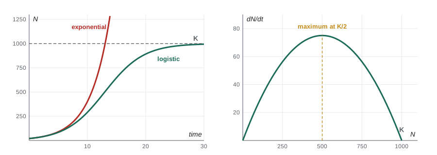
As a population becomes crowded, individuals compete for food, space or nesting sites, disease spreads more easily, and predators may concentrate on the abundant prey. Birth rates fall and death rates rise. These effects are called density-dependent because their strength depends on population density. The simplest model of density dependence, the logistic model introduced by Pierre-François Verhulst in 1838, assumes that the per capita growth rate declines in a straight line as the population approaches the carrying capacity, \( K \), the largest population the environment can support indefinitely:

When \( N \) is small, the term in brackets is close to 1 and growth is nearly exponential. As \( N \) approaches \( K \), the term approaches zero and growth stops. Plotted against time, the population follows an S-shaped (sigmoid) curve. The population grows fastest at \( N = K/2 \), where the product of numbers and per capita rate is greatest. That point is the basis of the maximum sustainable yield used in managing fisheries and game: a harvest equal to the growth rate at \( K/2 \), which is \( rK/4 \), can in theory be taken indefinitely. In practice, setting harvests at the theoretical maximum has repeatedly led to collapse, because \( r \) and \( K \) are uncertain and vary from year to year, as the collapse of Atlantic cod off Newfoundland in the early 1990s showed.

import numpy as np
from scipy.optimize import curve_fit

def logistic(t, K, r, N0):
    return K / (1 + (K - N0) / N0 * np.exp(-r * t))

# Invented census data: sheep introduced to an island (counts by year)
rng = np.random.default_rng(208)
years = np.arange(0, 26, 2)
true = logistic(years, 1700, 0.45, 50)
counts = np.round(true * rng.normal(1, 0.06, years.size))
(K, r, N0), _ = curve_fit(logistic, years, counts, p0=[1500, 0.3, 50])
for y, c in zip(years, counts):
    print(f"year {y:2d}: {int(c):5d}")
print(f"fitted K = {K:.0f}, r = {r:.3f} per year, N0 = {N0:.0f}")
print(f"maximum growth at N = K/2 = {K/2:.0f}; MSY = rK/4 = {r*K/4:.0f} per year")

year  0:    49
year  2:   107
year  4:   242
year  6:   552
year  8:   862
year 10:  1201
year 12:  1545
year 14:  1441
year 16:  1682
year 18:  1620
year 20:  1884
year 22:  1735
year 24:  1626
fitted K = 1713, r = 0.427 per year, N0 = 56
maximum growth at N = K/2 = 856; MSY = rK/4 = 183 per year

Time lags, cycles and chaos

The logistic model assumes that a population responds instantly to its own density. Real populations often respond with a delay: the number of young born this year may depend on how much food was available last year, or on the density when their parents were growing up. A delay of roughly a generation can make a population overshoot its carrying capacity, then crash below it, producing oscillations. Robert May showed in the 1970s that even a very simple discrete-time version of logistic growth, appropriate for species that breed once a year, can produce stable equilibria, regular cycles or chaos, depending only on how fast the population grows.

def discrete_logistic(rd, K=100, N0=10, years=30):
    N = [N0]
    for _ in range(years):
        n = N[-1]
        N.append(max(n + rd * n * (1 - n / K), 0))
    return N

for rd in (0.5, 1.8, 2.3, 2.7):
    traj = discrete_logistic(rd)
    tail = ", ".join(f"{x:5.1f}" for x in traj[-8:])
    print(f"rd = {rd}:  last 8 years -> {tail}")

rd = 0.5:  last 8 years -> 100.0, 100.0, 100.0, 100.0, 100.0, 100.0, 100.0, 100.0
rd = 1.8:  last 8 years -> 100.0, 100.0, 100.0, 100.0, 100.0, 100.0, 100.0, 100.0
rd = 2.3:  last 8 years -> 118.2,  68.8, 118.2,  68.8, 118.2,  68.8, 118.2,  68.8
rd = 2.7:  last 8 years -> 126.5,  36.0,  98.2, 102.9,  94.8, 108.1,  84.4, 120.0

With a low growth rate (0.5), the population approaches 100 smoothly. At 1.8 it overshoots and the oscillations dampen. At 2.3 it settles into a stable two-point cycle, alternating between high and low years. At 2.7 the pattern never repeats: this is deterministic chaos, in which the next value is fully determined by the current one, yet tiny differences in starting conditions grow until long-term prediction is impossible. The lesson for ecologists is that irregular fluctuations in a population do not necessarily mean that the environment is fluctuating; they can arise from the population's own dynamics.

Density-independent factors

Not everything that kills organisms depends on how crowded they are. A late spring frost, a flood, a severe drought or an early blizzard can kill a large fraction of a population regardless of its density. These density-independent factors cause fluctuations but cannot by themselves regulate a population, because they do not push it back toward any particular size. In many insects of temperate regions, weather explains most year-to-year changes in abundance, while density-dependent factors such as parasitoids and disease set the long-run level around which populations fluctuate. A long debate among ecologists in the mid-twentieth century over whether populations are controlled mainly by weather or by density has been resolved by recognizing that both act together.

Small populations and chance

Deterministic models assume that births and deaths happen at exactly their average rates. In small populations, chance matters. Demographic stochasticity is randomness in the fates of individuals: by bad luck, all the chicks hatched in a year might be male. Environmental stochasticity is randomness in conditions from year to year, such as good and bad seasons, which affects all individuals together. Even a population with a positive average growth rate can go extinct by chance if it is small and its growth rate varies a lot. This is why conservation biologists estimate a minimum viable population and use population viability analysis, covered in BIOL-367.

import numpy as np

def extinction_prob(N0, mean_r, sd_r, years=50, reps=5000, seed=208):
    rng = np.random.default_rng(seed)
    extinct = 0
    for _ in range(reps):
        N = N0
        for _ in range(years):
            lam = np.exp(rng.normal(mean_r, sd_r))
            N = rng.poisson(N * lam)          # demographic noise
            if N == 0:
                extinct += 1
                break
    return extinct / reps

for N0 in (5, 20, 80):
    p = extinction_prob(N0, mean_r=0.01, sd_r=0.25)
    print(f"start {N0:3d} individuals: probability of extinction within 50 years = {p:.3f}")

start   5 individuals: probability of extinction within 50 years = 0.777
start  20 individuals: probability of extinction within 50 years = 0.448
start  80 individuals: probability of extinction within 50 years = 0.137

Small populations face a further risk called the Allee effect, after the ecologist Warder Clyde Allee: below some density, individuals do worse rather than better, because they cannot find mates, cooperate in defence or feed effectively. Colonial seabirds and many marine invertebrates that spawn into the water need large numbers to breed successfully. Allee effects create a threshold below which a population tends to decline to extinction, a danger for species reduced to a few individuals.

Regulation in real populations

Field studies show that density dependence is common but rarely as simple as the logistic model. In song sparrows on Mandarte Island, British Columbia, studied for decades, the number of young produced per female falls steeply as the population grows, because territories become crowded. In plants, crowding causes self-thinning: as seedlings in a dense stand grow, many die, and the survivors grow larger, so that the number of plants falls as mean plant mass rises along a predictable line. In many mammals, density dependence acts through juvenile survival, while adult survival stays high. Lesson 5 shows how life tables separate these effects by age.