
AI-480 · Lesson 8 of 12 · 25 min
Tensor, sequence, context and expert parallelism
Data parallelism and sharding divide the batch: every device still runs every layer on its own examples. When individual layers become too large, when the batch per device becomes too small to hide communication, or when sequences become so long that one device cannot hold their activations, the work inside each layer must be divided as well. This is model parallelism within a layer, and it comes in several forms. Tensor parallelism splits the weight matrices of each layer across devices. Sequence and context parallelism split the tokens of each sequence. Expert parallelism places different experts of a mixture-of-experts model on different devices. This lesson explains each, the communication each requires, and where in the cluster each belongs.
Splitting a matrix multiplication
Consider a layer computing \(Y = XA\), where \(X\) holds activations for a batch of tokens and \(A\) is a weight matrix. There are two natural ways to split \(A\) across \(t\) devices:
- Column parallelism: split \(A\) by columns into \([A_1, A_2, \ldots, A_t]\). Each device computes \(Y_i = XA_i\), a slice of the output's columns. The input \(X\) must be available on every device, and the output ends up split.
- Row parallelism: split \(A\) by rows and \(X\) by columns correspondingly. Each device computes a partial product \(X_iA_i\) of full output size, and the true output is the sum \(Y = \sum_i X_iA_i\), which requires an all-reduce.
The insight of Megatron-LM, introduced by Shoeybi and colleagues at NVIDIA in 2019, was to chain these so that communication is needed only once per block.
Megatron tensor parallelism
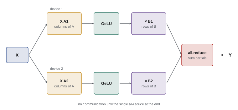
A transformer MLP computes \(Y = \text{GeLU}(XA)\,B\). Megatron splits \(A\) by columns and \(B\) by rows. Each device computes \(\text{GeLU}(XA_i)\) independently, which is valid because GeLU acts elementwise on the column slice, then multiplies by its rows \(B_i\) to obtain a partial output. A single all-reduce sums the partial outputs. The self-attention block is split the same way: attention heads are divided among devices, so the query, key and value projections are column-parallel, each device computes attention for its heads, and the output projection is row-parallel, followed by one all-reduce. Each transformer layer therefore needs two all-reduces in the forward pass and two in the backward pass, each of an activation tensor of size \(s \times b \times h\).
import numpy as np
rng = np.random.default_rng(0)
def gelu(x):
    return 0.5 * x * (1 + np.tanh(0.7978845608 * (x + 0.044715 * x**3)))
# Megatron-style tensor parallel MLP on t devices
tokens, h, t = 6, 8, 4
X = rng.standard_normal((tokens, h))
A = rng.standard_normal((h, 4 * h)); B = rng.standard_normal((4 * h, h))
reference = gelu(X @ A) @ B
A_parts = np.split(A, t, axis=1)          # column-parallel first matrix
B_parts = np.split(B, t, axis=0)          # row-parallel second matrix
partial = [gelu(X @ A_parts[i]) @ B_parts[i] for i in range(t)]   # no communication needed so far
Y = np.sum(partial, axis=0)               # one all-reduce of the outputs
print("tensor-parallel MLP matches:", np.allclose(Y, reference))
print("weights per device:", A_parts[0].size + B_parts[0].size, "of", A.size + B.size)
# Mixture of experts: top-2 routing with a capacity limit
n_tokens, n_experts, k, capacity_factor = 64, 8, 2, 1.25
logits = rng.standard_normal((n_tokens, n_experts)) + np.linspace(0, 1.5, n_experts)   # skewed router
top = np.argsort(-logits, axis=1)[:, :k]
counts = np.bincount(top.ravel(), minlength=n_experts)
capacity = int(capacity_factor * n_tokens * k / n_experts)
dropped = np.maximum(counts - capacity, 0).sum()
print("tokens per expert:", counts.tolist(), " capacity:", capacity)
print(f"assignments over capacity (dropped or rerouted): {dropped} of {n_tokens*k}")
# Load-balancing auxiliary loss (Switch Transformer form): n * sum(f_i * p_i)
probs = np.exp(logits) / np.exp(logits).sum(axis=1, keepdims=True)
f = counts / counts.sum(); p = probs.mean(axis=0)
print(f"balance loss: {n_experts * np.sum(f * p):.3f} (1.000 when perfectly balanced)")tensor-parallel MLP matches: True weights per device: 128 of 512 tokens per expert: [6, 3, 6, 14, 16, 19, 25, 39] capacity: 20 assignments over capacity (dropped or rerouted): 24 of 128 balance loss: 1.277 (1.000 when perfectly balanced)
The first part of the output confirms that splitting the MLP across four devices and summing their partial outputs reproduces the full result exactly, while each device stores a quarter of the weights. The second part, discussed later in this lesson, shows how an unbalanced router overloads some experts.
Where tensor parallelism belongs
Tensor parallelism communicates activations within every layer, in the critical path: the next operation cannot start until the all-reduce finishes. Its communication volume per layer is proportional to \(sbh\) and does not shrink as more devices are added, while computation per device does. It therefore needs very fast links and is almost always confined to the GPUs within one server, connected by NVLink at hundreds of gigabytes per second, typically with a tensor-parallel degree of 2, 4 or 8. Larger NVLink domains, such as NVIDIA's GB200 NVL72 rack, which joins 72 GPUs in one NVLink fabric, allow larger tensor-parallel and expert-parallel groups. Tensor parallelism also needs large hidden dimensions to keep each device's matrix slices big enough for efficient kernels.
Worked problem
Tensor-parallel communication cost
A model with hidden size 8,192 is trained with tensor parallelism of degree 8 on one server, with micro-batches of 1 sequence of 4,096 tokens in BF16. Each all-reduce runs at an effective 300 GB/s. Estimate the tensor-parallel communication time per layer for forward and backward passes.
Show solution
- Activation tensor size: \(4096 \times 1 \times 8192 \times 2\) bytes = 67 MB.
- Ring all-reduce traffic per device: \(2 \times (7/8) \times 67\) MB ≈ 117 MB.
- Time per all-reduce: \(117 \times 10^6 / 300 \times 10^9 \approx 0.39\) ms.
- Four all-reduces per layer (two forward, two backward): about 1.6 ms.
Answer: About 1.6 ms per layer; compared with the layer's compute of a few milliseconds, this is significant, which is why tensor parallelism stays on NVLink and why overlapping these collectives with computation is an active area of optimization.
Sequence parallelism
Tensor parallelism splits the matrix multiplications, but the operations between them, layer normalization and dropout, run on the full activation tensor on every device, duplicating both work and activation memory. Sequence parallelism, introduced by Korthikanti and colleagues in 2022, splits these operations along the sequence dimension instead: each of the \(t\) tensor-parallel devices handles \(s/t\) tokens for normalization and dropout. The all-reduce at the end of each tensor-parallel block is replaced by a reduce-scatter (leaving the output split by sequence) and the input to the next block is reassembled with an all-gather. Since a reduce-scatter plus an all-gather costs the same as an all-reduce, communication is unchanged, but the duplicated activations are divided by \(t\). Combined with selective recomputation, this reduced activation memory by about five times in the original experiments.
Context parallelism for long sequences
Training on long contexts, hundreds of thousands or millions of tokens, creates activations too large for one device even with FlashAttention and tensor parallelism. Context parallelism splits each sequence into chunks across devices for the whole layer, not just the normalization. Most of a transformer layer acts on each token independently, so chunks can be processed separately; attention is the exception, because every query must see the keys and values of earlier tokens. Ring attention, described by Liu and colleagues in 2023, arranges the devices in a ring: each device computes attention between its queries and its local key-value block, then passes the key-value block to the next device while receiving one from the previous device, overlapping communication with computation until every query has seen every relevant block. An alternative, DeepSpeed-Ulysses, uses all-to-all communication to switch from splitting by sequence to splitting by attention heads for the attention computation, then switches back. With causal masking, chunks must be assigned carefully, for example pairing early and late chunks, so that devices have equal work.
Mixture-of-experts models
A mixture-of-experts (MoE) layer replaces a transformer's single MLP with many expert MLPs and a small router that sends each token to only a few of them, typically the top one or two by router score. The model can thus have far more parameters than it uses for any single token. Mixtral 8x7B, released by Mistral AI in 2023, has 8 experts per layer and routes each token to 2, for about 47 billion total but 13 billion active parameters. DeepSeek-V3 has 671 billion parameters with 37 billion active per token, using 256 routed experts and one shared expert per layer. Training compute scales with active parameters, so MoE models deliver the quality of a larger model for the training cost of a smaller one, at the price of much more memory and complex communication.
Expert parallelism
Expert parallelism places different experts on different devices. In each MoE layer, every device routes its tokens, then an all-to-all exchange sends each token to the devices holding its chosen experts; the experts process the tokens they receive; and a second all-to-all returns the outputs to the tokens' original devices. All-to-all traffic is proportional to the number of tokens and the hidden size, and is sensitive to network topology, because every device talks to every other. Systems therefore keep expert-parallel groups within fast domains where possible, limit how many nodes each token may be routed to, as DeepSeek-V3 does, and overlap all-to-all communication with computation of other micro-batches.
Load balance is the second challenge. If the router sends most tokens to a few popular experts, those devices become stragglers while others sit idle, and if experts have a fixed capacity, excess tokens are dropped or passed through unchanged. A capacity factor sets each expert's buffer as a multiple of the average load. The code example shows a skewed router: one expert receives 39 assignments against a capacity of 20, and 24 of 128 assignments exceed capacity. Training adds an auxiliary load-balancing loss, such as \(n \sum_i f_i p_i\) from the Switch Transformer paper, where \(f_i\) is the fraction of tokens sent to expert \(i\) and \(p_i\) its mean router probability; it equals 1 when routing is uniform and rises with imbalance. DeepSeek-V3 instead adjusts a bias on each expert's router score during training to steer load without an auxiliary loss.
| Strategy | What is split | Main collective | Typical placement |
|---|---|---|---|
| Tensor parallelism | Weight matrices within layers | All-reduce of activations, per layer | Within a server (NVLink) |
| Sequence parallelism | Norm and dropout activations by token | Reduce-scatter and all-gather | Same group as tensor parallelism |
| Context parallelism | Whole sequence into chunks | Point-to-point ring or all-to-all | Within or across nearby servers |
| Expert parallelism | Experts of MoE layers | All-to-all of tokens | Within fast domains, limited node spread |
Overlapping tensor-parallel communication
Because tensor-parallel collectives sit in the critical path, recent systems work hard to overlap them with computation. One approach decomposes the matrix multiplication that follows an all-gather into chunks, so that the multiplication of the first chunk starts while the next chunk is still arriving; the same idea applies to a reduce-scatter following a multiplication. Libraries implement these collective matrix multiplications with fine-grained synchronization between communication and compute kernels. Another approach runs two micro-batches in an interleaved fashion, so that one micro-batch's communication overlaps the other's computation. These techniques can hide much of the tensor-parallel communication shown in the example above, making larger tensor-parallel degrees practical.
Combining intra-layer strategies
In large training systems these strategies are combined. A typical large dense model might use 8-way tensor parallelism with sequence parallelism within each server, context parallelism for long-context training phases, and pipeline and data parallelism across servers. A large mixture-of-experts model might use tensor parallelism for the attention layers and expert parallelism for the expert layers, with different group sizes for each, since attention and expert layers have different communication patterns. Frameworks such as Megatron-Core, DeepSpeed and JAX-based systems provide configurable implementations, but choosing the combination still requires understanding the memory and communication arithmetic of each.
Common mistakes
MistakeRunning tensor parallelism across slow inter-server links.
InsteadKeep tensor-parallel groups within NVLink domains.
MistakeUsing high tensor-parallel degrees on small models.
InsteadEnsure matrix slices stay large enough for efficient kernels.
MistakeIgnoring duplicated activations in tensor-parallel layers.
InsteadAdd sequence parallelism.
MistakeTraining MoE without load balancing.
InsteadUse an auxiliary loss or bias adjustment and set capacity.
MistakeAssigning causal sequence chunks naively.
InsteadBalance early and late chunks across devices.
Summary and key terms
- Column- and row-parallel splits divide matrix multiplications across devices.
- Megatron tensor parallelism needs two all-reduces per layer in each pass.
- Tensor parallelism communicates in the critical path and belongs on NVLink.
- Sequence parallelism splits normalization and dropout, saving activation memory.
- Context parallelism splits long sequences, using ring attention or all-to-all.
- MoE models activate a few experts per token, decoupling parameters from compute.
- Expert parallelism uses all-to-all routing and needs load balancing.
- Tensor parallelism
- Splitting layer weight matrices across devices.
- Column parallelism
- Splitting a weight matrix by output columns.
- Row parallelism
- Splitting a weight matrix by input rows.
- Sequence parallelism
- Splitting non-matmul activations by token.
- Context parallelism
- Splitting whole sequences across devices.
- Ring attention
- Passing key-value blocks around a ring of devices.
- Mixture of experts
- Layer routing tokens to a few of many experts.
- Active parameters
- Parameters used for each token.
- Expert parallelism
- Placing experts on different devices.
- Capacity factor
- Expert buffer size relative to average load.
Practice problems
Work each problem on paper first, then reveal the answer to check.
Which split of A lets GeLU run without communication?
Show answer
Column parallelism.
How many all-reduces does a Megatron layer need in the forward pass?
Show answer
Two: attention and MLP.
Why is tensor parallelism kept within a server?
Show answer
It communicates in every layer in the critical path.
Activation tensor size for s = 2,048, b = 2, h = 4,096 in BF16?
Show answer
33.5 MB.
What does sequence parallelism replace each all-reduce with?
Show answer
A reduce-scatter and an all-gather.
Why can most of a layer run on sequence chunks independently?
Show answer
It acts on each token separately; only attention mixes tokens.
What passes around the ring in ring attention?
Show answer
Key-value blocks.
Mixtral 8x7B total and active parameters?
Show answer
About 47B total, 13B active.
Which collective does expert parallelism use?
Show answer
All-to-all.
Value of the Switch balance loss for uniform routing?
Show answer
1.
Lesson quiz · 5 questions
Score 60% or more to complete this lesson.
Create a free account to save your progress, take quizzes and earn a certificate.