
AI-480 · Lesson 6 of 12 · 25 min
Data parallelism and collective communication
Data parallelism is the oldest, simplest and still most widely used way to train on many devices. Every device holds a complete copy of the model; each processes a different slice of the training batch; and after the backward pass the devices average their gradients so that every copy applies the same update and the replicas stay identical. Mathematically, the result is the same as training on one enormous device with the whole batch. The engineering challenge is communication: every step, each device must exchange a volume of data roughly equal to twice the size of the model's gradients. This lesson covers the collective communication operations that distributed training is built on, the ring and tree algorithms that implement them, the cost model used to predict their speed, how frameworks overlap communication with computation, and the optimization issues raised by very large batches.
Synchronous data parallelism
In synchronous data-parallel training with \(N\) workers, each training step proceeds as follows. The global batch of \(B\) examples is split into \(N\) shards of \(B/N\). Each worker runs the forward and backward passes on its shard, producing a local gradient \(g_i\). The workers then compute the average gradient \(\bar{g} = \frac{1}{N}\sum_i g_i\), which equals the gradient of the loss on the whole batch, and each applies the identical optimizer update. Because the loss is an average over examples, the averaged gradient is exactly the full-batch gradient, so data parallelism changes the speed of training but not its mathematics. Random seeds for dropout and data order must be managed per worker so that shards are distinct.
Earlier systems, such as Google's DistBelief (2012), used parameter servers: dedicated machines held the parameters, workers pushed gradients to them and pulled updated weights, often asynchronously. Asynchronous updates avoided waiting for slow workers but introduced stale gradients that could harm convergence. Modern large-scale training almost always uses synchronous updates with collective communication among the workers themselves.
Collective operations
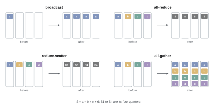
Collective operations involve every member of a group of devices. The core set, provided by libraries such as NVIDIA's NCCL, AMD's RCCL and the Message Passing Interface (MPI), is:
- Broadcast: one device sends the same data to all others, for example initial weights.
- Reduce: data from all devices is combined, typically summed, onto one device.
- All-reduce: data from all devices is summed and the result delivered to every device. This is the collective of data parallelism.
- Reduce-scatter: data is summed, but each device receives only one shard of the result.
- All-gather: each device contributes one shard and every device receives the concatenation of all shards.
- All-to-all: each device sends a different piece of data to every other device, used in expert parallelism (Lesson 8).
An all-reduce is equivalent to a reduce-scatter followed by an all-gather, a decomposition that both explains the ring algorithm and underlies sharded data parallelism in Lesson 7.
The ring all-reduce
A naive all-reduce that sends every gradient to one device and back would overload that device's links. The ring algorithm, popularized for deep learning by Baidu in 2017 and adopted in Horovod and NCCL, arranges the \(N\) devices in a logical ring and splits the data into \(N\) chunks. In the reduce-scatter phase, each device sends one chunk to its neighbour and adds the chunk it receives to its own copy; after \(N-1\) steps, each device holds the complete sum of one chunk. In the all-gather phase, the completed chunks travel around the ring for another \(N-1\) steps until every device has them all. Each device sends and receives \(2(N-1)/N\) times the data size, which approaches twice the data size and, crucially, does not grow with the number of devices. Every link is busy in every step, so the ring uses the network's bandwidth fully.
import numpy as np
# Ring all-reduce among N workers: reduce-scatter, then all-gather
def ring_allreduce(grads):
    n = len(grads)
    chunks = [np.array_split(g.copy(), n) for g in grads]
    sent = 0
    # reduce-scatter: after n-1 steps, worker i holds the full sum of chunk (i+1) mod n
    for step in range(n - 1):
        msgs = [(i, (i - step) % n, chunks[i][(i - step) % n].copy()) for i in range(n)]
        for i, c, data in msgs:
            dst = (i + 1) % n
            chunks[dst][c] = chunks[dst][c] + data; sent += data.size
    # all-gather: pass the completed chunks around the ring
    for step in range(n - 1):
        msgs = [(i, (i + 1 - step) % n, chunks[i][(i + 1 - step) % n].copy()) for i in range(n)]
        for i, c, data in msgs:
            chunks[(i + 1) % n][c] = data; sent += data.size
    return [np.concatenate(c) for c in chunks], sent
rng = np.random.default_rng(0)
size = 1200
for n in (2, 4, 8):
    grads = [rng.standard_normal(size) for _ in range(n)]
    out, sent = ring_allreduce(grads)
    exact = np.sum(grads, axis=0)
    ok = all(np.allclose(o, exact) for o in out)
    per_worker = sent / n
    print(f"N={n}: correct={ok}  values sent per worker={per_worker:.0f}  formula 2(N-1)/N*S={2*(n-1)/n*size:.0f}")
# Time model for all-reducing BF16 gradients of a 7B model
S = 7e9 * 2                    # bytes
for n, bw in [(8, 450e9), (64, 50e9), (1024, 50e9)]:
    t = 2 * (n - 1) / n * S / bw
print(f"N={n:5d}, link {bw/1e9:4.0f} GB/s: all-reduce takes {t:.2f} s")N=2: correct=True values sent per worker=1200 formula 2(N-1)/N*S=1200 N=4: correct=True values sent per worker=1800 formula 2(N-1)/N*S=1800 N=8: correct=True values sent per worker=2100 formula 2(N-1)/N*S=2100 N= 8, link 450 GB/s: all-reduce takes 0.05 s N= 64, link 50 GB/s: all-reduce takes 0.55 s N= 1024, link 50 GB/s: all-reduce takes 0.56 s
The traffic per worker matches the formula and approaches twice the gradient size as workers are added, so the bandwidth term of the all-reduce time is almost independent of scale. Communicating 14 GB of BF16 gradients over 50 GB/s network links takes over half a second whether there are 64 workers or 1,024. With 450 GB/s NVLink inside a server, the same operation takes about 50 milliseconds.
A cost model for collectives
Communication time is usually modelled with two parameters: a latency \(\alpha\) per message, covering software overhead and the time for the first byte to arrive, and an inverse bandwidth \(\beta\) per byte. Sending \(S\) bytes costs \(\alpha + \beta S\). For the ring all-reduce:
The bandwidth term is nearly constant in \(N\), but the latency term grows linearly, because the ring needs \(2(N-1)\) sequential steps. For large gradient buffers bandwidth dominates; for small messages on thousands of devices latency dominates. Tree-based algorithms, such as the double binary trees that NCCL uses for large clusters, need only about \(2\log_2 N\) latency steps while still using bandwidth well, and hierarchical algorithms first reduce within each server over NVLink, then across servers over the network, then broadcast within each server. NCCL chooses among algorithms and protocols automatically based on message size and topology.
Worked problem
Latency or bandwidth?
With \(\alpha = 5\) µs and links of 50 GB/s, estimate the ring all-reduce time for (a) a 1 MB buffer on 1,024 GPUs and (b) a 1 GB buffer on 1,024 GPUs.
Show solution
- Latency term for N = 1,024: \(2 \times 1023 \times 5\) µs ≈ 10.2 ms.
- Bandwidth term (a): \(2 \times (1023/1024) \times 10^6 / (50 \times 10^9)\) ≈ 40 µs.
- Total (a): about 10.3 ms, dominated by latency.
- Bandwidth term (b): \(2 \times 10^9 / (50 \times 10^9)\) ≈ 40 ms; total about 50 ms, dominated by bandwidth.
Answer: The small buffer takes about 10 ms, almost all latency; the large one takes about 50 ms, mostly bandwidth. Small messages should be grouped into larger buckets, or a tree algorithm used.
Overlapping communication with computation
Waiting for a full all-reduce after the backward pass would leave the accelerators idle. Instead, frameworks overlap the two. Gradients become available layer by layer during backpropagation, last layer first, so communication can begin for the final layers while earlier layers are still computing. PyTorch's DistributedDataParallel (DDP) groups gradients into buckets, 25 MB by default, and launches an asynchronous all-reduce as soon as each bucket is complete. Bucketing amortizes latency over many gradients, and overlapping hides most of the communication time behind computation. If communication takes longer than the backward pass, the excess is exposed and lowers MFU. Gradient accumulation (Lesson 5) also helps: gradients need to be all-reduced only once per optimizer step, not once per micro-batch.
Communication can also be made cheaper. Gradients can be sent in BF16 rather than FP32, halving traffic. Gradient compression methods, such as top-k sparsification, low-rank approximation (PowerSGD) and 1-bit quantization with error feedback, shrink messages further, though they add computation and can affect convergence. Low-communication methods, such as local SGD and DiLoCo, let workers take many local steps between synchronizations, which is attractive when workers are connected by slow links, for example across data centres.
Large-batch training
Data parallelism increases the global batch size as workers are added, unless each worker's share shrinks. Larger batches give more accurate gradient estimates but fewer optimizer steps per epoch, and beyond a point they stop speeding up training. Important findings include:
- The linear scaling rule: Goyal and colleagues at Facebook (2017) trained ResNet-50 on ImageNet in one hour with a batch of 8,192 images on 256 GPUs, scaling the learning rate in proportion to the batch size and using a gradual warm-up.
- Layer-wise adaptive optimizers: LARS and LAMB adapt the step size for each layer, allowing batches of tens of thousands; LAMB trained BERT in 76 minutes.
- The critical batch size: McCandlish and colleagues at OpenAI (2018) showed that each task has a batch size, related to the noise in its gradients, beyond which larger batches give diminishing returns. The critical batch grows as training progresses and the loss falls, which is why large language model runs often increase the batch size during training.
Large language models are commonly trained with global batches of a few million tokens. A run on 16,384 GPUs with a 16-million-token batch gives each GPU only about 1,000 tokens per step, which is one reason very large runs must combine data parallelism with other forms of parallelism instead of adding ever more replicas.
| Aspect | Effect of adding data-parallel workers |
|---|---|
| Compute per worker per step | Falls in proportion (for a fixed global batch) |
| Communication per worker per step | About 2 × gradient size, nearly constant |
| Memory per worker | Unchanged: full model state on every worker |
| Global batch size | Grows if per-worker batch is kept constant |
| Sensitivity to slow workers | Grows: each step waits for the slowest worker |
Stragglers and synchronization
In synchronous training, every step waits for the slowest worker. A single GPU running hot and throttling its clock, a server with a degraded network link, or a worker whose data loader stalls slows the entire job. At thousands of devices, the chance that some worker is slow at any moment becomes high. Monitoring per-worker step times, detecting and replacing slow nodes, and keeping input pipelines well ahead of the accelerators are all part of operating data-parallel training at scale (Lesson 11).
Initialization and consistency
Data-parallel replicas must start from identical parameters and stay identical. Frameworks broadcast the initial weights from one rank to all others at start-up, and every replica applies the same averaged gradient with the same optimizer, so replicas remain synchronized as long as their arithmetic is deterministic. Subtle bugs can break this: a layer whose buffers, such as batch normalization statistics, are updated locally and never synchronized, or a random operation seeded differently on each rank where it should be identical. Periodically comparing parameter checksums across replicas catches such drift early.
Common mistakes
MistakeAssuming data parallelism reduces memory per device.
InsteadEach replica still holds the full model state; use sharding for that.
MistakeAll-reducing each small gradient separately.
InsteadBucket gradients to amortize latency.
MistakeAll-reducing after every micro-batch.
InsteadAll-reduce once per optimizer step with gradient accumulation.
MistakeScaling the batch without adjusting the learning rate or warm-up.
InsteadRetune learning rate schedules for larger batches.
MistakeAdding workers past the critical batch size.
InsteadCombine with model parallelism instead.
Summary and key terms
- Data parallelism replicates the model and splits each batch across workers.
- Averaging gradients reproduces the full-batch gradient exactly.
- Collectives include broadcast, all-reduce, reduce-scatter, all-gather and all-to-all.
- Ring all-reduce sends about twice the data per worker, independent of N.
- The α–β model separates latency from bandwidth costs.
- Bucketing and overlap hide communication behind the backward pass.
- Very large batches give diminishing returns beyond the critical batch size.
- Data parallelism
- Replicating the model and splitting the batch.
- All-reduce
- Sum across devices delivered to every device.
- Reduce-scatter
- Sum across devices, each receiving one shard.
- All-gather
- Every device receives all devices' shards.
- Ring algorithm
- Collective passing chunks around a logical ring.
- NCCL
- NVIDIA Collective Communications Library.
- Gradient bucket
- Group of gradients communicated together.
- Parameter server
- Machine holding parameters for workers.
- Linear scaling rule
- Scaling learning rate with batch size.
- Critical batch size
- Batch beyond which returns diminish.
Practice problems
Work each problem on paper first, then reveal the answer to check.
Why does gradient averaging give the full-batch gradient?
Show answer
The loss is an average over examples.
Which two collectives make up an all-reduce?
Show answer
Reduce-scatter then all-gather.
Data sent per worker in a ring all-reduce of S bytes over 16 workers?
Show answer
2 × 15/16 × S ≈ 1.875 S.
How many sequential steps does a ring all-reduce take?
Show answer
2(N − 1).
Bandwidth time to all-reduce 2 GB over 25 GB/s links?
Show answer
About 2 × 2 / 25 = 0.16 s.
Why do trees help on large clusters?
Show answer
Fewer latency steps, about 2 log₂ N.
What does DDP bucketing achieve?
Show answer
Amortizes latency and enables overlap.
Name two gradient compression methods.
Show answer
Top-k sparsification, PowerSGD, 1-bit quantization.
What did the linear scaling rule pair with to train ResNet-50 quickly?
Show answer
Gradual learning rate warm-up.
Why does one slow worker matter?
Show answer
Synchronous steps wait for the slowest worker.
Lesson quiz · 5 questions
Score 60% or more to complete this lesson.
Create a free account to save your progress, take quizzes and earn a certificate.