
AI-480 · Lesson 3 of 12 · 25 min
TPUs, systolic arrays and other AI accelerators
GPUs dominate AI training, but they are not the only option. Google has trained its models on its own Tensor Processing Units (TPUs) for a decade; Amazon, Meta, Microsoft and others design custom chips; start-ups have built wafer-sized processors and chips made almost entirely of on-die memory; and AMD and Intel compete directly with NVIDIA's GPUs. All of these designs respond to the same observation: neural network workloads are dominated by dense linear algebra in reduced precision, with predictable data flow, so silicon spent on general-purpose flexibility can instead be spent on arithmetic and memory bandwidth. This lesson explains the systolic array at the heart of many accelerators, the TPU family and its pod-scale design, the main alternative accelerators, and the software ecosystems that often matter as much as the hardware when choosing a platform.
Specialization and its trade-offs
Every chip design trades generality for efficiency. A CPU can run any program reasonably well. A GPU runs data-parallel programs very well and remains fully programmable. An application-specific integrated circuit (ASIC) for AI, such as a TPU, fixes much of the data flow in hardware, gaining energy efficiency and density at the cost of flexibility. Field-programmable gate arrays (FPGAs) sit in between: their logic can be reconfigured after manufacture, which suits low-latency inference and network processing but rarely matches ASIC or GPU density for large training jobs. Because a chip takes two to four years to design and must then serve for several more, AI accelerators bet on what workloads will look like years ahead. Chips that specialized too narrowly, for example on convolutional networks just as transformers took over, have struggled.
The systolic array
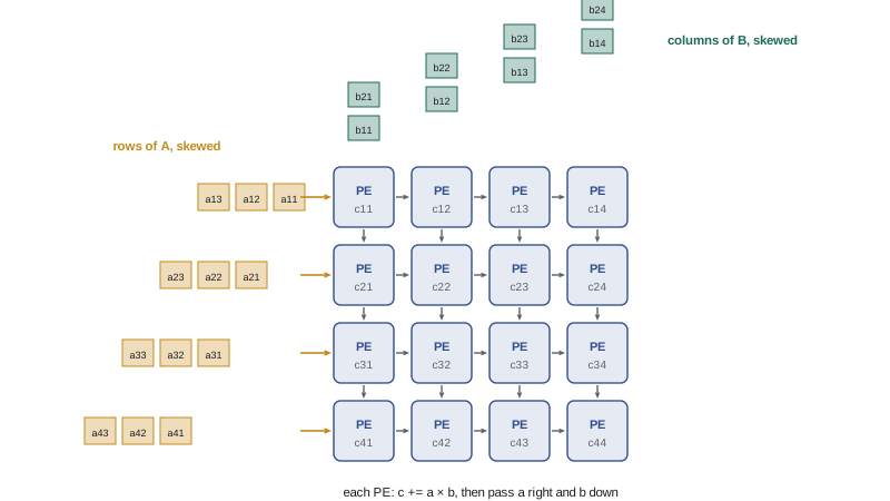
A systolic array is a grid of simple processing elements (PEs), each of which multiplies two numbers, adds the product to an accumulator, and passes its inputs to its neighbours on the next clock cycle. Data pulses through the grid rhythmically, like blood through the body, which gave the design its name when H. T. Kung and Charles Leiserson described it in 1978. In an output-stationary array computing \(C = AB\), each PE owns one element of \(C\); rows of \(A\) flow in from the left and columns of \(B\) flow in from the top, skewed by one cycle per row or column so that matching elements meet at the right PE at the right time. In a weight-stationary array, used by the first TPU, the weights are loaded into the PEs and stay there while activations stream through.
The key advantage is data reuse without memory traffic: each value read from memory is used by an entire row or column of PEs, passed hand to hand through short wires. A 128 × 128 array performs 16,384 multiply-accumulates per cycle while reading only 256 new values from its buffers. The cost is a fill and drain time: the array takes about \(m + n\) cycles to fill and empty, so it is efficient only when the shared dimension \(k\) is long.
import numpy as np
# Cycle-by-cycle simulation of an output-stationary systolic array
# PE (i, j) keeps a running sum for C[i, j]; A values flow right, B values flow down
def systolic_matmul(A, B):
    m, k = A.shape; k2, n = B.shape
    acc = np.zeros((m, n)); a_reg = np.zeros((m, n)); b_reg = np.zeros((m, n))
    cycles = 0
    for t in range(m + n + k - 2):
        # shift: each PE passes its A value right and its B value down
        a_reg[:, 1:] = a_reg[:, :-1].copy(); b_reg[1:, :] = b_reg[:-1, :].copy()
        # feed skewed inputs at the edges: row i of A is delayed by i cycles
        for i in range(m):
            s = t - i
            a_reg[i, 0] = A[i, s] if 0 <= s < k else 0.0
        for j in range(n):
            s = t - j
            b_reg[0, j] = B[s, j] if 0 <= s < k else 0.0
        acc += a_reg * b_reg
        cycles += 1
    return acc, cycles
rng = np.random.default_rng(0)
A = rng.integers(-3, 4, (4, 6)).astype(float); B = rng.integers(-3, 4, (6, 4)).astype(float)
C, cycles = systolic_matmul(A, B)
print("matches numpy:", np.allclose(C, A @ B))
print(f"4x4 array, k=6: {cycles} cycles for {4*4*6} multiply-accumulates on 16 PEs")
for k in (6, 64, 1024):
    A = rng.random((4, k)); B = rng.random((k, 4))
    _, cyc = systolic_matmul(A, B)
print(f"k={k:5d}: cycles={cyc:5d} ideal={k:5d} utilization={k/cyc:.0%}")matches numpy: True 4x4 array, k=6: 12 cycles for 96 multiply-accumulates on 16 PEs k= 6: cycles= 12 ideal= 6 utilization=50% k= 64: cycles= 70 ideal= 64 utilization=91% k= 1024: cycles= 1030 ideal= 1024 utilization=99%
The simulation shows the fill and drain overhead: with a short inner dimension of 6, half the cycles are spent filling and emptying the array, but with an inner dimension of 1,024 utilization reaches 99 %. Real accelerators keep their arrays busy by streaming long sequences of tiles back to back, overlapping one tile's drain with the next tile's fill.
The TPU family
Google began deploying TPUs in its data centres in 2015, initially for inference. The first TPU used a 256 × 256 array of 8-bit integer multiply-accumulators, delivering 92 tera-operations per second with a thermal design power of about 75 W. TPU v2 (2017) added floating point and training support, introducing the BF16 format that later spread across the industry, and connected chips into pods with a dedicated inter-chip interconnect. TPU v4 (2021) delivered about 275 teraFLOP/s of BF16 per chip with 32 GB of HBM, and joined 4,096 chips into a pod using a three-dimensional torus network whose links pass through optical circuit switches, which can reconfigure the topology and route around failed racks. Later generations, including v5p, Trillium (v6) and Ironwood (v7), increased per-chip throughput, memory and pod size further.
Each TPU chip contains one or more TensorCores, each with large matrix multiply units (systolic arrays of 128 × 128 in recent generations), a vector unit for elementwise work, and a scalar unit for control. Rather than many independently scheduled threads, a TPU is programmed through a compiler, XLA, which takes a whole computation graph, decides the layout of every tensor, fuses operations and schedules data movement explicitly. This static, compiler-driven approach makes TPUs very efficient on large, regular workloads but less forgiving of dynamic shapes and custom operations.
Other accelerators
The accelerator landscape is broad and changes quickly. Representative designs include:
- AMD Instinct GPUs: the MI300X (2023) combines GPU chiplets with 192 GB of HBM3 at 5.3 TB/s, more memory than contemporary NVIDIA GPUs, programmed through the ROCm software stack and HIP, a CUDA-like language.
- Cloud provider chips: Amazon's Trainium and Inferentia, Microsoft's Maia and Meta's MTIA are custom accelerators designed for their owners' workloads and offered mainly inside their own clouds.
- Intel Gaudi: accelerators with matrix engines and integrated Ethernet ports for scale-out networking.
- Cerebras: the Wafer-Scale Engine uses an entire silicon wafer as one chip, with hundreds of thousands of cores and tens of gigabytes of on-chip SRAM, avoiding off-chip memory traffic for models that fit.
- SRAM-centric inference chips: designs such as Groq's LPU keep model weights in on-chip SRAM across many chips and schedule execution deterministically, targeting very low latency token generation.
- Edge and mobile neural processing units (NPUs): small accelerators in phones, laptops and cameras that run compressed models within a few watts.
| Design | Core idea | Strengths | Limitations |
|---|---|---|---|
| GPU (NVIDIA, AMD) | Many programmable SMs with tensor cores | Flexible, mature software, wide availability | Power hungry; general features cost area |
| TPU | Large systolic arrays, compiler-scheduled | Efficient at scale, integrated pod network | Mainly available through one cloud; prefers static graphs |
| Wafer-scale | Whole wafer with on-chip SRAM | Huge on-chip bandwidth | Limited memory capacity, specialized software |
| SRAM-centric inference | Weights held on chip, deterministic schedule | Very low latency per token | Many chips per model; less suited to training |
| Edge NPU | Small integer and low-precision engines | Low power, on-device privacy | Small models only |
Software ecosystems
Hardware without mature software is of little use. NVIDIA's CUDA platform, with libraries such as cuBLAS, cuDNN and NCCL, and deep integration in PyTorch, has been refined since 2007 and is a major reason for NVIDIA's dominance. Competing platforms reduce the gap in several ways: compilers such as XLA (used by JAX and TensorFlow, and by PyTorch through PyTorch/XLA) target TPUs and other chips; OpenAI's Triton language lets developers write high-performance kernels in Python that compile for NVIDIA and AMD GPUs; and the PyTorch 2 compiler stack can lower models to different backends. When evaluating an accelerator, engineers ask practical questions: Do the models and operations we need run correctly? How much engineering effort does porting take? Are the communication libraries and distributed training frameworks mature? Can we hire people who know the platform?
Choosing hardware
Hardware choice depends on the workload and the organization. Key factors include the performance on the actual models, measured as time to train or cost per token rather than peak FLOP/s; memory capacity and bandwidth, which decide how many chips a model needs; the network and how far the platform scales; software maturity; availability and lead times, which have been severe constraints during periods of high demand; total cost of ownership, including power and cooling; and strategic considerations such as dependence on a single supplier. Many organizations use more than one platform, for example training on GPUs or TPUs and serving on cheaper inference chips.
Worked problem
Comparing accelerators on cost per useful FLOP
Accelerator X costs $2.50 per hour, has a peak of 900 TFLOP/s and achieves 45 % MFU on your model. Accelerator Y costs $1.60 per hour, has a peak of 450 TFLOP/s and achieves 55 % MFU. Which is cheaper per unit of useful training work?
Show solution
- Useful throughput X: \(900 \times 0.45 = 405\) TFLOP/s.
- Useful throughput Y: \(450 \times 0.55 = 247.5\) TFLOP/s.
- Useful FLOPs per hour X: \(405 \times 10^{12} \times 3600 = 1.46 \times 10^{18}\); cost per \(10^{18}\) FLOPs: $2.50 / 1.46 ≈ $1.71.
- Useful FLOPs per hour Y: \(247.5 \times 10^{12} \times 3600 = 8.91 \times 10^{17}\); cost per \(10^{18}\) FLOPs: $1.60 / 0.891 ≈ $1.80.
Answer: X is slightly cheaper per useful FLOP ($1.71 versus $1.80 per 10¹⁸ FLOPs) and finishes faster, despite its higher hourly price.
Dataflow choices in accelerators
Accelerator designers choose which data stays put and which moves. In a weight-stationary design, each processing element holds a weight while inputs and partial sums flow past, which minimizes weight reads and suits inference with fixed weights. In an output-stationary design, as in the simulation above, each element accumulates one output while inputs and weights flow, minimizing the movement of partial sums. Row-stationary and other hybrid dataflows, explored in research chips such as MIT's Eyeriss, balance the movement of all three. The best choice depends on layer shapes, batch sizes and the relative energy cost of moving data, which in modern chips far exceeds the energy of the arithmetic itself: reading a value from off-chip DRAM can cost hundreds of times more energy than a multiply-accumulate. Much of accelerator design is therefore the design of memory hierarchies and data movement rather than arithmetic units.
Chiplets and packaging
As single chips approach the maximum size that lithography can print, about 800 square millimetres, accelerators increasingly combine several smaller dies, or chiplets, in one package. AMD's MI300X joins compute chiplets on top of input-output dies; NVIDIA's Blackwell B200 joins two large dies with a 10 TB/s chip-to-chip link so that software sees one GPU. Advanced packaging technologies, such as TSMC's CoWoS, place the dies and HBM stacks side by side on a silicon interposer with thousands of fine connections. Packaging capacity, together with HBM supply, has at times limited how many accelerators could be produced, showing that the bottlenecks of AI hardware extend well beyond the design of the chip itself.
Benchmarks
Independent benchmarks help compare platforms. MLPerf, run by the MLCommons consortium, publishes training and inference results for standard tasks, including large language model pre-training and fine-tuning, on systems submitted by vendors and cloud providers, with rules that make results comparable. MLPerf results show both per-chip performance and how well systems scale to thousands of accelerators. They remain only a guide, since a team's own models, sequence lengths and software stack may behave differently, but they are a useful check on marketing claims.
Common mistakes
MistakeComparing accelerators by peak FLOP/s alone.
InsteadCompare measured time or cost to train your workload.
MistakeIgnoring the software ecosystem.
InsteadCheck model support, kernels, libraries and porting effort.
MistakeFeeding systolic arrays short matrices.
InsteadKeep inner dimensions long to amortize fill and drain.
MistakeAssuming one chip suits training and serving equally.
InsteadMatch hardware to each workload's bottleneck.
MistakeOverlooking memory capacity.
InsteadMore memory per chip can mean fewer chips and less communication.
Summary and key terms
- Accelerators trade flexibility for efficiency in dense, low-precision linear algebra.
- Systolic arrays pass data between neighbouring PEs, reusing each value many times.
- Systolic arrays need long inner dimensions to amortize fill and drain.
- TPUs combine large systolic arrays, compiler scheduling with XLA and pod-scale networks.
- Alternatives include AMD GPUs, cloud provider chips, wafer-scale engines and SRAM-centric chips.
- Software ecosystems strongly influence which hardware is practical.
- Choose hardware by measured cost and time on real workloads.
- ASIC
- Chip designed for a specific application.
- FPGA
- Reconfigurable logic chip.
- Systolic array
- Grid of PEs passing data to neighbours each cycle.
- Processing element
- Simple multiply-accumulate unit in an array.
- Weight-stationary
- Dataflow keeping weights fixed in the PEs.
- TPU
- Google's Tensor Processing Unit.
- XLA
- Compiler for linear algebra graphs used by TPUs and JAX.
- Optical circuit switch
- Reconfigurable optical link switch used in TPU pods.
- NPU
- Neural processing unit, often in edge devices.
- ROCm
- AMD's GPU software platform.
Practice problems
Work each problem on paper first, then reveal the answer to check.
Why do accelerators favour reduced precision?
Show answer
Smaller arithmetic units give more throughput per area and watt.
How does a systolic array reduce memory traffic?
Show answer
Values pass between PEs and are reused many times.
How many MACs per cycle does a 128 × 128 array perform?
Show answer
16,384.
What limits systolic array utilization for short inner dimensions?
Show answer
Fill and drain cycles.
What numerical format did TPU v2 introduce?
Show answer
BF16.
How do TPU v4 pods route around failed racks?
Show answer
Optical circuit switches reconfigure the torus.
Why are TPUs less forgiving of dynamic shapes?
Show answer
XLA compiles static graphs and layouts.
Name one advantage of the MI300X.
Show answer
192 GB of HBM3.
What is Triton?
Show answer
A Python-based language for writing GPU kernels.
Name three factors in choosing hardware.
Show answer
Measured performance, memory, network, software, availability, cost.
Lesson quiz · 5 questions
Score 60% or more to complete this lesson.
Create a free account to save your progress, take quizzes and earn a certificate.