
AI-480 · Lesson 12 of 12 · 25 min
Energy, cost and the economics of compute
Every technique in this course ultimately serves one goal: getting the most useful training and inference out of a fixed budget of money, energy and time. Compute has become one of the main inputs to AI progress and one of its largest costs. Frontier training runs cost hundreds of millions of dollars; AI data centres are being planned at the scale of hundreds of megawatts to gigawatts; and the availability of chips, power and cooling now shapes which organizations can build which models. This final lesson brings the course together around economics and energy: how to estimate the energy, emissions and cost of a run, the choice between renting and owning hardware, the economics of inference, trends in compute and hardware efficiency, the policy context, and a capstone exercise in planning a complete training run.
Energy of a training run
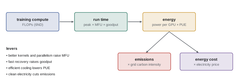
The energy of a run follows from its compute. Compute divided by the sustained throughput of the cluster gives the run time; multiplying the run time by the cluster's power draw gives the energy used by the IT equipment; and multiplying by the facility's power usage effectiveness (PUE), the ratio of total facility power to IT power, adds cooling, power conversion and other overheads. An H100 is rated at up to 700 W, but a training server also draws power for CPUs, memory, network adapters, switches and fans, so planners typically allow 1.1 to 1.4 kW per GPU at the server and network level. Modern AI data centres achieve PUEs of about 1.1 to 1.4, with liquid cooling increasingly required for the densest racks; the DCE courses cover these facilities in detail.
Here \(g\) is the goodput fraction from Lesson 11. The formula makes an important point plain: the number of GPUs \(N\) cancels out. For a fixed amount of compute, more GPUs finish sooner but use the same energy; what reduces energy is higher MFU and goodput, more efficient hardware, and a lower PUE.
import numpy as np
# Energy, cost and emissions of a training run
params, tokens = 70e9, 15e12
flops = 6 * params * tokens
gpus, peak, mfu, goodput = 8192, 989e12, 0.40, 0.90
seconds = flops / (gpus * peak * mfu * goodput)
gpu_hours = gpus * seconds / 3600
print(f"compute {flops:.2e} FLOPs -> {seconds/86400:.0f} days on {gpus} GPUs, {gpu_hours/1e6:.2f} million GPU-hours")
# Facility energy: GPU power plus host share, times PUE
watts_per_gpu = 700 * 0.85 + 550     # average GPU draw plus share of CPUs, memory, network, fans
pue = 1.2
energy_mwh = gpus * watts_per_gpu * pue * seconds / 3600 / 1e6
print(f"average facility power {gpus*watts_per_gpu*pue/1e6:.1f} MW, energy {energy_mwh:,.0f} MWh")
# Emissions on grids of different carbon intensity (g CO2e per kWh)
for grid, g in [("hydro-dominated grid", 30), ("mixed grid", 380), ("coal-heavy grid", 800)]:
    print(f"{grid:22s}: {energy_mwh*1000*g/1e6:8,.0f} tonnes CO2e")
# Cost: renting versus owning, in US dollars
rent = 2.50                           # dollars per GPU-hour
own_capex, years, util = 35000.0, 4, 0.80          # per GPU including its share of servers and network
power_price = 0.08                    # dollars per kWh
own_hourly = own_capex / (years * 8760 * util) + watts_per_gpu * pue / 1000 * power_price
print(f"rented: ${gpu_hours*rent/1e6:.1f}M   owned: ${own_hourly:.2f} per GPU-hour, ${gpu_hours*own_hourly/1e6:.1f}M")
# Inference: cost per million output tokens on one GPU
for tok_s in (1500, 6000):
print(f"serving at {tok_s} tokens/s per GPU: ${rent/(tok_s*3600)*1e6:.3f} per million tokens")compute 6.30e+24 FLOPs -> 25 days on 8192 GPUs, 4.92 million GPU-hours average facility power 11.3 MW, energy 6,753 MWh hydro-dominated grid : 203 tonnes CO2e mixed grid : 2,566 tonnes CO2e coal-heavy grid : 5,403 tonnes CO2e rented: $12.3M owned: $1.36 per GPU-hour, $6.7M serving at 1500 tokens/s per GPU: $0.463 per million tokens serving at 6000 tokens/s per GPU: $0.116 per million tokens
Training a 70B model on 15 trillion tokens, close to the recipe of Meta's Llama 3 70B, which Meta reported took about 6.4 million H100 GPU-hours, needs about \(6.3 \times 10^{24}\) FLOPs. At 40 % MFU and 90 % goodput, 8,192 GPUs take about 25 days and draw about 11 MW, using roughly 6,800 MWh, comparable to the annual electricity use of several hundred homes. Emissions depend almost entirely on where that electricity comes from, varying more than twentyfold between grids.
In Canada, grid carbon intensity varies widely by province: Quebec, Manitoba and British Columbia run largely on hydroelectricity, with intensities of a few to a few tens of grams of CO2e per kWh, while Alberta and Saskatchewan rely more on natural gas and coal, with intensities of several hundred grams per kWh. Siting a large training cluster on a low-carbon provincial grid can therefore cut a run's emissions by more than 90 %.
Beyond electricity: embodied carbon and water
Operational electricity is not the only environmental cost. Manufacturing chips, servers and buildings produces embodied emissions, which for accelerators can be a meaningful share of their lifetime footprint, especially when they run on clean power. Data centres also consume water, directly in evaporative cooling and indirectly through power generation, which matters in water-stressed regions. Responsible reporting of a model's environmental impact, as recommended by researchers such as Strubell, Luccioni and colleagues, includes the hardware used, GPU-hours, location, PUE and grid intensity, so that estimates can be checked and compared. The most effective reduction strategies are the efficiency techniques of this course, choice of location and time, and avoiding unnecessary training runs by reusing and fine-tuning existing models.
Renting versus owning
Organizations obtain compute in three main ways: renting on demand from a cloud provider, reserving capacity for a fixed term at a discount, or buying hardware and running it in their own or a colocation data centre. Renting avoids large upfront costs and lets a team scale up for one run and down afterwards; owning can be much cheaper per GPU-hour if the hardware stays busy, but requires capital, data centre space and power, operations staff, and acceptance of the risk that newer hardware will make it obsolete. The code example illustrates the comparison: at the assumed figures, an owned GPU kept 80 % busy for four years costs about $1.36 per hour including power, against $2.50 to rent, but only if it really is used that much. Cloud GPU prices have moved substantially as supply has changed: on-demand H100 prices that exceeded $8 per hour in 2023 had fallen to a few dollars by 2025 from many providers.
| Factor | Rent (cloud) | Own (on premises or colocation) |
|---|---|---|
| Upfront cost | None | Large capital outlay |
| Cost per GPU-hour at high utilization | Higher | Lower |
| Flexibility to scale | High, subject to capacity | Limited by what was bought |
| Access to newest hardware | Often early, at a premium | Requires new purchases |
| Operations burden | Mostly provider's | Team's, including failures and repairs |
| Risk of idle capacity | Low | High if workloads fall |
The economics of inference
For a widely used model, inference compute over its lifetime can far exceed training compute. Generating one token with a dense model costs about \(2N\) FLOPs, a third of the training cost per token, but a popular model may generate trillions of tokens per day. Inference economics are expressed as cost per million tokens, which depends on throughput per accelerator. Small-batch generation is memory-bound (Lesson 2), so serving systems batch many requests together to reuse each weight read across many tokens, a technique called continuous batching, and use quantization (Lesson 4), efficient KV-cache management (Lesson 5), speculative decoding, and sometimes specialized inference chips (Lesson 3). In the code example, raising throughput from 1,500 to 6,000 tokens per second per GPU cuts the cost from about $0.46 to $0.12 per million tokens. These economics also feed back into training decisions: they explain why teams train smaller models on far more data than compute-optimal (Lesson 1) and why mixture-of-experts models, with few active parameters, are attractive.
Worked problem
Lifetime compute: training versus inference
A 70B dense model is trained on 15 trillion tokens. After release it serves 100 billion tokens per day (input and output combined) for one year. Compare training and inference compute.
Show solution
- Training: \(6 \times 70 \times 10^9 \times 15 \times 10^{12} = 6.3 \times 10^{24}\) FLOPs.
- Inference per token: \(2 \times 70 \times 10^9 = 1.4 \times 10^{11}\) FLOPs.
- Tokens per year: \(10^{11} \times 365 = 3.65 \times 10^{13}\).
- Inference per year: \(1.4 \times 10^{11} \times 3.65 \times 10^{13} = 5.1 \times 10^{24}\) FLOPs.
Answer: One year of inference needs about 5.1 × 10²⁴ FLOPs, comparable to the 6.3 × 10²⁴ FLOPs of training; at higher usage, or over a longer life, inference dominates, and it typically runs at lower utilization, so its cost is higher still.
Trends in compute and efficiency
Several trends shape planning. Analyses by Epoch AI estimated that the compute used to train frontier models grew by roughly four to five times per year through the early 2020s, far faster than hardware improved, with the difference made up by larger clusters and larger budgets. Hardware price-performance, measured in FLOP/s per dollar, has improved more slowly, doubling roughly every two to three years, helped greatly by the move to lower precisions. Algorithmic progress, better architectures, data and training recipes, has also reduced the compute needed to reach a given level of performance. Energy has emerged as a binding constraint: a cluster of 100,000 current-generation GPUs needs on the order of 150 MW, and the largest planned AI campuses exceed a gigawatt, requiring new generation and transmission capacity that can take years to build.
Policy and supply
Advanced AI chips are now a subject of industrial and trade policy. Their manufacture is concentrated in a few companies and locations, especially leading-edge fabrication in Taiwan and high-bandwidth memory from a few suppliers, which makes supply sensitive to disruption. The United States has imposed export controls on advanced AI chips and chipmaking equipment since 2022, revising them several times, and other countries, including Canada, apply export controls through multilateral arrangements and national lists. Governments in both countries have also announced public investment in national AI compute capacity for researchers and companies. These policies change frequently, so engineers planning international deployments should check current rules with legal and compliance specialists.
Capstone: planning a training run
The capstone asks you to produce a complete plan for training a model, bringing together every lesson. Choose a model, for example a 30-billion-parameter dense transformer or a mixture-of-experts model with a stated number of active parameters, and a dataset size, then prepare:
- A compute estimate using \(6ND\) and a justified choice of tokens per parameter, considering inference cost (Lesson 1).
- A hardware choice with justification from throughput, memory and software ecosystem (Lessons 2 and 3).
- A numerical precision plan, including FP32 master weights and any FP8 use (Lesson 4).
- A memory budget per device covering model state, activations and recomputation (Lesson 5).
- A parallelism configuration with tensor, pipeline, data and sharding degrees, the micro-batch size, and expected bubble and communication time (Lessons 6 to 9).
- A cluster and network layout, storage requirements for data and checkpoints (Lesson 10).
- A reliability plan with a checkpoint interval, expected goodput and monitoring (Lesson 11).
- Estimates of run time, energy, emissions and cost, with a sensitivity analysis showing how MFU, goodput and location change them (this lesson).
Present the plan as a short design document with a table of key numbers, the assumptions behind each, and the main risks. A good plan is one that a team could start from, and that makes clear which measurements in the first days of the run would confirm or overturn its assumptions.
Common mistakes
MistakeAssuming more GPUs use less energy for the same run.
InsteadEnergy depends on compute, efficiency and PUE, not GPU count.
MistakeReporting emissions without location and grid data.
InsteadState hardware, GPU-hours, PUE and grid intensity.
MistakeComparing rent and own costs at full utilization only.
InsteadUse realistic utilization and include operations costs.
MistakeIgnoring inference when planning training.
InsteadWeigh lifetime serving cost in model size choices.
MistakeTreating chip supply and export rules as fixed.
InsteadCheck current availability and regulations before committing.
Summary and key terms
- Run energy follows from compute, MFU, goodput, power per GPU and PUE.
- For fixed compute, the number of GPUs does not change energy use.
- Emissions depend mostly on the electricity grid's carbon intensity.
- Owning hardware is cheaper per hour only at high utilization.
- Inference can exceed training compute over a model's life.
- Frontier compute has grown faster than hardware efficiency; power is a constraint.
- The capstone plan integrates compute, hardware, memory, parallelism, reliability and cost.
- PUE
- Power usage effectiveness: facility power over IT power.
- Carbon intensity
- Emissions per unit of electricity, g CO2e/kWh.
- Embodied emissions
- Emissions from manufacturing hardware and buildings.
- Total cost of ownership
- Full lifetime cost of owning hardware.
- Reserved capacity
- Compute rented for a fixed term at a discount.
- Cost per million tokens
- Inference cost measure.
- Continuous batching
- Serving many requests together as they arrive.
- Price-performance
- Compute delivered per dollar.
- Export controls
- Rules restricting transfer of sensitive technology.
- Sensitivity analysis
- Testing how results change with assumptions.
Practice problems
Work each problem on paper first, then reveal the answer to check.
Energy for 1,000 GPUs at 1.2 kW each, PUE 1.3, for 10 days?
Show answer
1,000 × 1.2 × 1.3 × 240 h = 374 MWh.
Why does GPU count cancel out of run energy?
Show answer
More GPUs run proportionally shorter for the same compute.
Emissions of 500 MWh at 50 g CO2e/kWh?
Show answer
25 tonnes.
Name two environmental costs besides operational electricity.
Show answer
Embodied emissions and water use.
Owned cost per hour for a $30,000 GPU over 3 years at 70 % use, ignoring power?
Show answer
30,000 / (3 × 8,760 × 0.7) ≈ $1.63.
Inference FLOPs per token for a 13B dense model?
Show answer
About 2.6 × 10¹⁰.
Cost per million tokens at $2 per hour and 2,000 tokens/s?
Show answer
$2 / 7.2 ≈ $0.28.
Why do MoE models suit inference economics?
Show answer
Few active parameters per token.
Roughly how much power does a 100,000-GPU cluster need?
Show answer
On the order of 150 MW.
Name four parts of the capstone plan.
Show answer
Compute, hardware, precision, memory, parallelism, network, reliability, cost.
Lesson quiz · 5 questions
Score 60% or more to complete this lesson.
Create a free account to save your progress, take quizzes and earn a certificate.