
AI-480 · Lesson 2 of 12 · 25 min
GPU architecture and the roofline model
Graphics processing units were built to shade millions of pixels in parallel, and that same design turned out to suit neural networks almost perfectly. Since AlexNet was trained on two consumer GPUs in 2012, NVIDIA and its competitors have reshaped the GPU around AI: adding tensor cores that multiply small matrices in a single instruction, stacking high-bandwidth memory beside the processor, and supporting ever-lower numerical precisions. To train models efficiently, an engineer needs to understand what is inside the chip, how work is scheduled onto it, where data lives, and why many operations are limited by memory bandwidth rather than arithmetic. This lesson covers the GPU's execution model, its compute units and memory hierarchy, the roofline model for reasoning about performance, and the kernel-level techniques, such as fusion and tiling, that close the gap between peak and achieved throughput.
Throughput versus latency
A CPU core is a latency machine: it tries to finish each instruction stream as quickly as possible using deep pipelines, branch prediction, out-of-order execution and large caches. A GPU is a throughput machine: it runs tens of thousands of threads at once and hides the latency of any one thread by switching to others that are ready. When one group of threads waits hundreds of cycles for memory, the hardware scheduler simply issues instructions from another group. This works only when there is plenty of independent work, which is why GPUs need large matrices and large batches to perform well, and why small or sequential workloads often run poorly on them.
The execution model
In NVIDIA's CUDA programming model, a program launches a kernel over a grid of thread blocks. Each block contains up to 1,024 threads that can cooperate through fast on-chip shared memory and synchronize with barriers. The hardware executes threads in groups of 32 called warps; all threads in a warp execute the same instruction at the same time on different data, a model NVIDIA calls single instruction, multiple threads (SIMT). If threads in a warp take different branches, the paths run one after another, a slowdown called warp divergence. AMD GPUs use a similar model, with 64-thread wavefronts in many designs, programmed through the HIP and ROCm software stack.
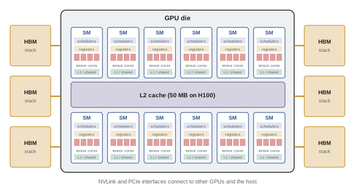
Thread blocks are assigned to streaming multiprocessors (SMs), the GPU's building blocks. An SM contains integer and floating-point arithmetic units, special function units for operations such as exponentials, load and store units, a large register file, tensor cores, and a block of memory that serves as L1 cache and programmer-managed shared memory. Several blocks can reside on one SM at once if registers and shared memory allow, and the fraction of the SM's thread slots in use is called occupancy.
Tensor cores
Tensor cores, introduced with the Volta architecture in 2017, perform a small matrix multiply-accumulate, such as \(D = A \times B + C\) on tiles of a few rows and columns, as a single operation. They deliver far more arithmetic per clock than ordinary floating-point units, but only for matrix operations in reduced precision: FP16 and BF16 with FP32 accumulation, TF32, FP8 on Hopper, and FP4 on Blackwell. On an H100, dense BF16 tensor core throughput is about 989 teraFLOP/s, while ordinary FP32 arithmetic on the same chip delivers about 67 teraFLOP/s. A workload that does not map onto tensor cores, or uses FP32 for its matrix multiplications, leaves most of the chip idle.
The memory hierarchy
Data moves through a hierarchy of memories that trade capacity for speed:
- Registers: the fastest storage, private to each thread; an H100 SM has a 256 KB register file.
- Shared memory and L1 cache: up to 256 KB per SM on H100, shared by the threads of a block, with bandwidth of tens of terabytes per second across the chip.
- L2 cache: 50 MB on H100, shared by all SMs.
- High-bandwidth memory (HBM): stacks of DRAM dies beside the GPU on a silicon interposer; 80 GB at about 3.35 TB/s on H100 SXM.
- Host memory and other GPUs: reached over PCIe (about 64 GB/s each way for PCIe 5.0 x16) or NVLink (900 GB/s total on H100).
Each level is roughly an order of magnitude slower than the one above. Efficient kernels keep data in registers and shared memory for as long as possible and read each value from HBM as few times as they can.
| Specification | A100 SXM (2020) | H100 SXM (2022) | B200 (2024) |
|---|---|---|---|
| Architecture | Ampere | Hopper | Blackwell |
| Dense BF16 tensor throughput | 312 TFLOP/s | 989 TFLOP/s | about 2,250 TFLOP/s |
| Lowest tensor precision | INT8 / INT4 | FP8 | FP4 |
| HBM capacity | 80 GB HBM2e | 80 GB HBM3 | 192 GB HBM3e |
| HBM bandwidth | 2.0 TB/s | 3.35 TB/s | about 8 TB/s |
| NVLink bandwidth per GPU | 600 GB/s | 900 GB/s | 1,800 GB/s |
| Maximum power | 400 W | 700 W | about 1,000 W |
Arithmetic intensity and the roofline
Whether an operation is limited by arithmetic or by memory depends on its arithmetic intensity: the number of floating-point operations performed per byte moved to or from memory. The roofline model, introduced by Williams, Waterman and Patterson in 2009, bounds attainable performance:
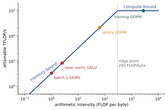
where \(I\) is arithmetic intensity in FLOP/byte and \(B_{\text{mem}}\) is memory bandwidth. Below the ridge point, \(I = P_{\text{peak}} / B_{\text{mem}}\), performance rises linearly with intensity and the kernel is memory-bound; above it, the kernel is compute-bound. For an H100 doing dense BF16 work, the ridge point is about 989 / 3.35 ≈ 295 FLOP per byte: a kernel must perform almost 300 operations for every byte it reads or writes to use the tensor cores fully.
Large matrix multiplications have high intensity because each element of the inputs is reused many times. For square \(n \times n\) matrices in BF16, intensity is about \(2n^3 / (3 \times 2n^2) = n/3\), so matrices larger than about 900 on a side can be compute-bound. Elementwise operations such as activation functions, residual additions and normalization perform only a few FLOPs per element and are firmly memory-bound.
import numpy as np
# Roofline model for an H100-class GPU (dense BF16)
peak = 989e12          # FLOP/s
bw = 3.35e12           # bytes/s of HBM bandwidth
ridge = peak / bw
print(f"ridge point: {ridge:.0f} FLOP per byte")
def matmul_intensity(m, k, n, bytes_per=2):
    flops = 2.0 * m * k * n
    traffic = bytes_per * (m * k + k * n + m * n)   # read A and B, write C once
    return flops, flops / traffic
cases = [("batch-1 decode GEMV", 1, 8192, 8192), ("small batch 16", 16, 8192, 8192),
         ("training GEMM", 8192, 8192, 8192), ("skinny 4096x64", 4096, 64, 4096)]
for name, m, k, n in cases:
    flops, ai = matmul_intensity(m, k, n)
    attain = min(peak, ai * bw)
    bound = "compute" if ai >= ridge else "memory"
    print(f"{name:20s} AI={ai:8.1f} FLOP/B  attainable={attain/1e12:6.1f} TFLOP/s  ({bound}-bound)")
# Elementwise operations are almost always memory-bound
n = 2**28
ai_gelu = (8.0 * n) / (2 * 2.0 * n)   # about 8 FLOPs per element, read and write BF16
print(f"GELU over {n:,} elements: AI={ai_gelu:.1f} FLOP/B, time at full bandwidth={4.0*n/bw*1e3:.2f} ms")ridge point: 295 FLOP per byte batch-1 decode GEMV AI= 1.0 FLOP/B attainable= 3.3 TFLOP/s (memory-bound) small batch 16 AI= 15.9 FLOP/B attainable= 53.4 TFLOP/s (memory-bound) training GEMM AI= 2730.7 FLOP/B attainable= 989.0 TFLOP/s (compute-bound) skinny 4096x64 AI= 62.1 FLOP/B attainable= 207.9 TFLOP/s (memory-bound) GELU over 268,435,456 elements: AI=2.0 FLOP/B, time at full bandwidth=0.32 ms
The batch-one matrix-vector product, the core of generating one token at a time during inference, reaches only about 3 TFLOP/s, a third of one percent of peak, because every weight is read from memory to be used just once. Training matrix multiplications with large batches sit comfortably on the roof. This contrast explains why inference is usually limited by memory bandwidth and training by compute, and why the two workloads favour different hardware and optimizations.
Kernel fusion and tiling
Two techniques do most of the work of moving kernels toward the roof. Kernel fusion combines several operations into one kernel so that intermediate results stay in registers or shared memory rather than travelling to HBM and back. Applying a bias, an activation function and dropout in one fused kernel, for example, reads and writes the tensor once instead of three times. Compilers such as XLA, PyTorch's torch.compile with its Triton backend, and TensorRT fuse operations automatically.
Tiling breaks a large operation into blocks that fit in shared memory and registers, so each block of input is loaded once and reused for many operations. High-performance matrix multiplication libraries such as cuBLAS and CUTLASS tile at several levels: thread blocks compute output tiles, warps compute sub-tiles, and tensor cores compute the smallest tiles. FlashAttention, introduced by Tri Dao and colleagues in 2022, applied tiling to attention: instead of writing the full sequence-by-sequence attention matrix to HBM, it computes attention block by block in shared memory with an online softmax, cutting memory traffic dramatically and making long contexts practical. Later versions exploit Hopper features such as asynchronous data movement and FP8.
Worked problem
Is this layer memory-bound?
A layer normalization reads a BF16 tensor of 64 million elements and writes the result, performing about 10 FLOPs per element. On an H100 (989 TFLOP/s, 3.35 TB/s), estimate the time if it is limited by memory and if it were limited by compute.
Show solution
- Bytes moved: read and write \(2 \times 64 \times 10^6 \times 2\) bytes = 256 MB.
- Memory time: \(0.256 \times 10^9 / 3.35 \times 10^{12} \approx 76\) µs.
- FLOPs: \(10 \times 64 \times 10^6 = 6.4 \times 10^8\).
- Compute time (even at full tensor-core rate): \(6.4 \times 10^8 / 9.89 \times 10^{14} \approx 0.65\) µs.
- Arithmetic intensity: 640 MFLOP / 256 MB = 2.5 FLOP/byte, far below the ridge point.
Answer: About 76 µs, set entirely by memory bandwidth; the arithmetic would take under 1 µs, so fusing it with neighbouring operations is the way to speed it up.
Other GPU features that matter for training
Several further features shape training performance. Asynchronous copy engines move data between HBM and shared memory, or between GPUs, while the SMs compute, allowing communication and computation to overlap. Hopper's tensor memory accelerator (TMA) moves multidimensional tiles with a single instruction. Structured sparsity support can double tensor core throughput for weights pruned to a 2:4 pattern, though it is used more in inference than training. Multi-Instance GPU (MIG) partitions one GPU into isolated slices for smaller jobs. And the GPU's power and clock management means that sustained throughput can fall below the rated peak when a chip reaches its power or thermal limit, which is one reason measured utilization varies between clusters.
Measuring what a kernel achieves
Profiling tools report how close each kernel comes to its limits. NVIDIA Nsight Compute, for example, measures a kernel's achieved FLOP/s, memory bandwidth, occupancy and the reasons its warps stalled, and can plot the kernel on a roofline chart. A matrix multiplication reaching 70 to 80 % of tensor-core peak is doing well; an elementwise kernel reaching 80 to 90 % of HBM bandwidth is doing well, even though its FLOP/s are tiny. The right question for any kernel is therefore not "how many FLOP/s?" but "how close is it to the roof that applies to it?" A kernel far below both roofs usually suffers from poor memory access patterns, such as reads that are not coalesced into large contiguous transactions, low occupancy, or too little work per launch.
Writing custom kernels
Most training code relies on vendor libraries and compilers, but performance-critical operations sometimes justify custom kernels. CUDA C++ gives complete control; libraries such as CUTLASS and CuTe provide reusable building blocks for tiled matrix operations; and Triton lets developers write block-level kernels in Python, handling many low-level details automatically. Custom kernels are common for attention variants, fused optimizer steps, normalization combined with other operations, and quantized matrix multiplication. They must be tested carefully against reference implementations, because subtle errors in indexing or numerical precision can silently corrupt training.
Common mistakes
MistakeJudging a kernel only by its FLOP count.
InsteadCompute its arithmetic intensity and compare with the ridge point.
MistakeRunning matrix multiplications in FP32 on tensor-core GPUs.
InsteadUse BF16, FP16, TF32 or FP8 with appropriate accumulation.
MistakeUsing tiny batches or matrices on a large GPU.
InsteadGive the GPU enough parallel work to fill its SMs.
MistakeWriting each elementwise step as a separate kernel.
InsteadFuse operations to avoid repeated HBM traffic.
MistakeAssuming inference and training bottlenecks are the same.
InsteadSmall-batch inference is usually memory-bound; training is compute-bound.
Summary and key terms
- GPUs are throughput machines that hide latency with massive parallelism.
- CUDA kernels run grids of thread blocks; warps of 32 threads execute together.
- Streaming multiprocessors contain arithmetic units, tensor cores, registers and shared memory.
- Tensor cores deliver most of the chip's throughput, in reduced precision.
- The memory hierarchy runs from registers to shared memory, L2, HBM and beyond.
- The roofline model bounds performance by peak compute or intensity times bandwidth.
- Fusion and tiling, as in FlashAttention, keep data on chip and raise utilization.
- Streaming multiprocessor
- A GPU's basic compute building block.
- Warp
- Group of 32 threads executing together.
- Thread block
- Group of threads sharing memory on one SM.
- Tensor core
- Unit performing small matrix multiply-accumulates.
- HBM
- High-bandwidth memory stacked beside the GPU.
- Shared memory
- Fast on-chip memory managed by the programmer.
- Arithmetic intensity
- FLOPs performed per byte of memory traffic.
- Ridge point
- Intensity where a kernel becomes compute-bound.
- Kernel fusion
- Combining operations into one kernel.
- Tiling
- Splitting work into blocks that fit on chip.
Practice problems
Work each problem on paper first, then reveal the answer to check.
Why does a GPU need many threads to perform well?
Show answer
It hides memory latency by switching between ready threads.
What is warp divergence?
Show answer
Threads in a warp taking different branches, serializing execution.
What operation does a tensor core perform?
Show answer
A small matrix multiply-accumulate.
Ridge point of a chip with 400 TFLOP/s and 2 TB/s?
Show answer
200 FLOP/byte.
Arithmetic intensity of a square BF16 matmul with n = 3,000?
Show answer
About n/3 = 1,000 FLOP/byte.
Is a residual addition memory- or compute-bound?
Show answer
Memory-bound.
Why is batch-one decoding slow per FLOP?
Show answer
Each weight is read from memory for one use.
What does kernel fusion avoid?
Show answer
Writing and re-reading intermediate tensors in HBM.
What did FlashAttention avoid materializing?
Show answer
The full attention matrix in HBM.
Name two levels of the GPU memory hierarchy.
Show answer
Registers, shared memory, L2, HBM.
Lesson quiz · 5 questions
Score 60% or more to complete this lesson.
Create a free account to save your progress, take quizzes and earn a certificate.