Mechanistic interpretability

Mechanistic interpretability aims to reverse-engineer neural networks: to identify the features they represent and the circuits, the specific chains of computation through weights and activations, that turn inputs into outputs, much as one might reverse-engineer a compiled program. The goal is ambitious, and complete understanding of a frontier model is far off, but the field has made substantial progress: researchers have identified circuits for specific behaviours in language models, explained why individual neurons are hard to interpret, and developed tools that extract millions of interpretable features from large models. This lesson covers the transformer as a set of interpretable parts, causal interventions such as activation patching, superposition, sparse autoencoders and dictionary learning, circuit tracing, and the prospects and limits of the approach for safety.

The transformer as interpretable parts

A transformer can be viewed as a residual stream, a vector for each token position that runs through the network, to which each attention head and each MLP layer reads from and adds. This view, developed in work on transformer circuits, makes components easier to analyse: an attention head moves information between token positions, an MLP layer transforms information at a position, and the output is read from the final residual stream. Small models can be analysed exactly. For example, induction heads, pairs of attention heads that implement a "look for the previous occurrence of the current token and copy what followed it" pattern, were identified as a key mechanism behind in-context learning, and their sudden formation during training coincides with a jump in in-context learning ability.

Causal interventions

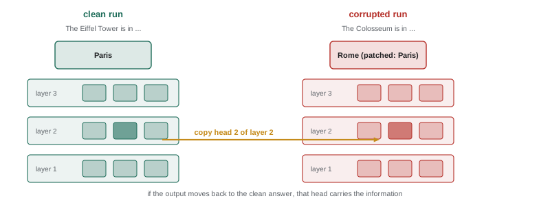
To show that a component matters for a behaviour, mechanistic interpretability relies on interventions rather than correlations. In activation patching (also called causal tracing or interchange intervention), the model is run on two inputs, a clean input where it behaves one way and a corrupted input where it behaves another, and activations from one run are copied into the other at a specific component. If patching a particular head's output from the clean run into the corrupted run restores the clean behaviour, that head carries the relevant information. Systematic patching across layers and positions maps where information flows. Ablation, setting a component's output to zero or to its mean, tests whether it is necessary. Using these tools, researchers have traced circuits for tasks such as identifying the indirect object in a sentence, recalling factual associations, and performing simple arithmetic.

Superposition

A recurring obstacle is that individual neurons are often polysemantic (Lesson 6). The superposition hypothesis, explored in toy models by Elhage and colleagues (2022), explains why: a network may need to represent more features than it has dimensions, and if each feature is sparse (rarely active), it can store them as nearly orthogonal directions in a lower-dimensional space, accepting a little interference when several happen to be active at once. Neurons then do not correspond to features; each feature is a direction spread across many neurons, and each neuron participates in many features. This makes neuron-by-neuron interpretation misleading, and it suggests a different approach: find the feature directions themselves.

Sparse autoencoders and dictionary learning

If activations are sparse combinations of many feature directions, then dictionary learning can recover those directions: find an overcomplete set of directions (more than the number of dimensions) such that each activation vector is well approximated by a combination of only a few of them. Sparse autoencoders (SAEs) do this with a neural network trained to reconstruct activations through a wide, sparsely active hidden layer. Anthropic's 2023 work applied SAEs to a small transformer and found features far more interpretable than neurons, and its 2024 work scaled the method to a production model, extracting millions of features, including features for specific people, places, programming concepts, deception, sycophancy and dangerous content, some of which could steer the model's behaviour when amplified. Other labs have published similar results and open tools.

import numpy as np
from sklearn.decomposition import PCA, DictionaryLearning

# Superposition in miniature: 8 sparse features stored in a 4-dimensional activation space
rng = np.random.default_rng(7)
n_feat, dim, n = 8, 4, 1500
directions = rng.normal(size=(n_feat, dim))
directions /= np.linalg.norm(directions, axis=1, keepdims=True)
active = rng.random((n, n_feat)) < 0.06                         # each feature is rarely active
coeffs = active * rng.uniform(0.5, 1.5, (n, n_feat))
acts = coeffs @ directions + rng.normal(0, 0.01, (n, dim))      # what we observe: 4-dim activations

def recovery(components):
    comps = components / np.linalg.norm(components, axis=1, keepdims=True)
    sims = np.abs(directions @ comps.T)                          # cosine similarity, true vs learned
    return sims.max(axis=1)

pca = PCA(n_components=dim).fit(acts)
dl = DictionaryLearning(n_components=n_feat, alpha=0.05, max_iter=60, random_state=0,
                        transform_algorithm="lasso_lars").fit(acts)
print("Best cosine match for each true feature direction:")
print("  PCA (4 orthogonal components):  ", " ".join(f"{s:.2f}" for s in recovery(pca.components_)))
print("  Sparse dictionary (8 atoms):    ", " ".join(f"{s:.2f}" for s in recovery(dl.components_)))
codes = dl.transform(acts[:500])
print(f"Average number of active dictionary atoms per example: {(np.abs(codes) > 1e-3).sum(axis=1).mean():.2f}")
print(f"Average number of truly active features per example:   {active[:500].sum(axis=1).mean():.2f}")

Best cosine match for each true feature direction:
  PCA (4 orthogonal components):   0.88 0.74 0.81 0.66 0.69 0.83 0.76 0.85
  Sparse dictionary (8 atoms):     0.90 1.00 1.00 1.00 0.97 0.99 0.99 1.00
Average number of active dictionary atoms per example: 0.84
Average number of truly active features per example:   0.44

In this toy setting, eight features are packed into four dimensions. PCA can find only four orthogonal directions, so each true feature matches its closest principal component only partially (cosine similarities around 0.66 to 0.88). Sparse dictionary learning, allowed eight directions and a sparsity penalty, recovers the true feature directions almost exactly (similarities of 0.90 to 1.00), and represents each example with less than one active atom on average, close to the true sparsity. Real SAEs work on activations with thousands of dimensions and millions of features, but the principle is the same: sparsity makes superposed features recoverable.

Circuits and attribution graphs

Features alone describe what a model represents; circuits describe how features combine to produce behaviour. Recent methods replace the model's MLP layers with interpretable approximations (such as transcoders or cross-layer transcoders) and trace how features at one layer activate features at the next for a specific input, producing attribution graphs of the computation behind an output. Studies using these tools have shown models planning ahead (for example selecting a rhyming word before writing the line that ends with it), performing multi-step reasoning internally, and, in some cases, producing explanations of their reasoning that do not match the internal computation, an important finding for the faithfulness of chain-of-thought explanations (Lesson 10). These analyses typically explain only part of the computation for a given prompt and require substantial human effort.

Interpretability for safety

Mechanistic interpretability offers potential safety applications that behavioural testing cannot provide:

• Detecting hidden objectives or deceptive reasoning by finding features associated with them, even when behaviour looks benign.
• Auditing for backdoors and data poisoning by identifying unusual features and circuits.
• Monitoring in deployment: watching for activation of safety-relevant features (such as features related to deception or dangerous knowledge) as a complement to output monitoring.
• Verifying that safety training changed the relevant mechanism, rather than just suppressing a behaviour superficially.
• Providing evidence in safety cases about what a model is and is not doing.

Limitations are significant. Dictionary features may not fully capture the model's computation (reconstruction errors can hide important information), interpretations of features are themselves hypotheses that need testing, coverage of a frontier model's behaviour remains partial, and methods require large amounts of computation and expert time. The field's trajectory is promising, but it does not yet provide the comprehensive guarantees that a safety case for a highly capable system would ideally need.

Automated interpretability

A frontier model may contain millions of sparse autoencoder features and vast numbers of possible circuits, far too many for researchers to inspect by hand. Automated interpretability uses language models to help: a model reads the top-activating examples of a feature and proposes a description, and a second step tests the description by asking a model to predict, from the description alone, how strongly the feature will activate on new text. The correlation between predicted and actual activations gives a score for how well the explanation captures the feature. Agents have also been built that run interpretability experiments themselves, choosing inputs, patching activations and refining hypotheses.

Automation makes interpretability scale, but it brings its own risks: generated descriptions can be confidently wrong or too broad, and scores based on top-activating examples may miss behaviour at weaker activation levels. Human review of samples and causal tests remain necessary.

Open problems

Researchers have highlighted several open problems that determine how far mechanistic interpretability can support safety:

• Dark matter: a significant fraction of model activations is not explained by current dictionaries, and important computations may hide there.
• Feature splitting and universality: features change with dictionary size, splitting into finer variants, which raises the question of which level of description is the right one.
• Scaling circuit analysis from single prompts to general mechanisms that explain behaviour across many inputs.
• Linking internal mechanisms to the high-level properties that matter for safety, such as intentions, goals and deception, which may not correspond to simple features.

Despite these open problems, the field has moved quickly from toy models to production systems in only a few years, and interpretability tools are already used in pre-deployment audits of frontier models. Their role in safety cases (Lesson 12) is likely to grow as coverage improves and methods are validated.