Generalization: bias, variance and learning theory

A model is useful only if it performs well on data it has not seen. Training minimizes error on the training set, but what we care about is the error on the whole distribution the data comes from. This lesson studies the gap between the two. It decomposes prediction error into bias, variance and noise; uses concentration inequalities to say how much a test set can be trusted; introduces the classical theory that bounds generalization by model complexity; and confronts the puzzle that modern networks, with far more parameters than training examples, generalize well anyway, including the phenomenon of double descent.

Training error, test error and the gap

Let a model \(h\) have loss \(\ell(h(\mathbf{x}), y)\). Its true risk is the expected loss over the data distribution, \(R(h) = \mathbb{E}[\ell(h(\mathbf{x}), y)]\), and its empirical risk is the average over \(n\) training examples, \(\hat{R}(h) = \frac{1}{n}\sum_{i}\ell(h(\mathbf{x}_{i}), y_{i})\). Learning chooses \(h\) to make \(\hat{R}\) small; the generalization gap \(R(h) - \hat{R}(h)\) measures how much that choice overfits the particular sample. Because \(h\) was chosen using the training data, \(\hat{R}(h)\) is a biased, optimistic estimate of \(R(h)\); an independent test set gives an unbiased one (AI-110, Lesson 9).

The bias–variance decomposition

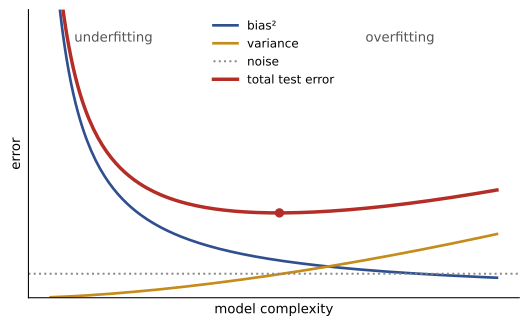
For squared loss, the expected error of a learning method at a point \(x\), averaged over random training sets and noise, splits into three parts. If \(y = f(x) + \varepsilon\) with noise variance \(\sigma^{2}\), and \(\hat{f}\) is the model learned from a random training set,

• Bias: the error of the average model, due to the model being too simple to represent \(f\).
• Variance: how much the model changes from one training set to another, due to fitting the particular noise in each sample.
• Noise: irreducible error that no model can remove.

import numpy as np

rng = np.random.default_rng(11)
f = lambda x: np.sin(2 * np.pi * x)
x_test = np.linspace(0.05, 0.95, 50)
n, sigma, trials = 30, 0.3, 500

print("degree   bias^2   variance   noise   total test MSE")
for deg in [1, 3, 7]:
    preds = np.empty((trials, x_test.size))
    for t in range(trials):
        x = rng.uniform(0, 1, n)
        y = f(x) + rng.normal(0, sigma, n)
        preds[t] = np.polyval(np.polyfit(x, y, deg), x_test)
    bias2 = np.mean((preds.mean(axis=0) - f(x_test)) ** 2)
    var = np.mean(preds.var(axis=0))
    print(f"{deg:>6} {bias2:8.3f} {var:10.3f} {sigma**2:7.3f} {bias2 + var + sigma**2:12.3f}")

degree   bias^2   variance   noise   total test MSE
     1    0.154      0.019   0.090        0.263
     3    0.003      0.014   0.090        0.107
     7    0.000      0.109   0.090        0.199

The straight line has large bias (it cannot bend to follow a sine) and small variance. The cubic has almost no bias and small variance: the best total. The degree-7 polynomial also has negligible bias, but its variance is several times larger, because with only 30 points it fits each sample's noise. Regularization, more data, simpler models and averaging (ensembles, bagging) all reduce variance; richer models and better features reduce bias.

How much can a test set be trusted?

Test accuracy is itself a random estimate. If a model's true accuracy is \(p\) and the test set has \(n\) independent examples, the measured accuracy has standard error \(\sqrt{p(1 - p)/n}\) (AI-110, Lesson 4). Concentration inequalities give guarantees that hold whatever the distribution. Hoeffding's inequality for the average of \(n\) independent values in \([0, 1]\) states

so a test set of \(n \ge \ln(2/\delta)/(2\varepsilon^{2})\) examples guarantees error at most \(\varepsilon\) with probability at least \(1 - \delta\).

import numpy as np

eps, delta = 0.02, 0.05
n_needed = int(np.ceil(np.log(2 / delta) / (2 * eps**2)))
print(f"Hoeffding: n >= ln(2/delta) / (2 eps^2) = {n_needed} test examples for +/-{eps} with 95% confidence")

rng = np.random.default_rng(12)
true_acc = 0.87
estimates = rng.binomial(n_needed, true_acc, size=100_000) / n_needed
print(f"Simulated: {np.mean(np.abs(estimates - true_acc) <= eps):.4f} of estimates within +/-{eps}")
for n in [100, 1000, 10000]:
    se = np.sqrt(true_acc * (1 - true_acc) / n)
    print(f"n = {n:>5}: standard error of accuracy {se:.4f}, 95% interval about +/-{1.96 * se:.3f}")

Hoeffding: n >= ln(2/delta) / (2 eps^2) = 4612 test examples for +/-0.02 with 95% confidence
Simulated: 1.0000 of estimates within +/-0.02
n =   100: standard error of accuracy 0.0336, 95% interval about +/-0.066
n =  1000: standard error of accuracy 0.0106, 95% interval about +/-0.021
n = 10000: standard error of accuracy 0.0034, 95% interval about +/-0.007

Hoeffding's bound is conservative, because it ignores the actual variance, but it needs no assumptions. The practical lesson is that differences of a fraction of a percent between models are meaningless on test sets of a few thousand examples; claims of improvement need test sets large enough, or repeated evaluations, to resolve them.

Complexity and generalization bounds

Why does a model chosen from a richer set of candidates overfit more? Suppose the learner picks from a finite set of \(|\mathcal{H}|\) hypotheses. Applying Hoeffding to each and a union bound over all of them gives, with probability at least \(1 - \delta\), for every \(h \in \mathcal{H}\):

The gap grows with the logarithm of the number of hypotheses and shrinks as \(1/\sqrt{n}\). For infinite hypothesis classes, such as all linear classifiers, \(\ln|\mathcal{H}|\) is replaced by a measure of capacity, the VC dimension (equal to \(d + 1\) for linear classifiers in \(d\) dimensions) or the Rademacher complexity. The message of classical learning theory is that you need more data than your model has effective capacity.

Selection is training: overfitting the test set

Every choice made by looking at data is a form of training. If many models, features or hyperparameter settings are tried and the best on the test set is reported, the test set has been used to select among \(|\mathcal{H}|\) options, and the reported score is optimistic by an amount that grows with the number of tries.

import numpy as np

rng = np.random.default_rng(14)
n_test = 500
y_test = rng.integers(0, 2, n_test)                       # labels: pure coin flips
best = 0.0
for k in range(1, 1001):                                  # try 1,000 useless "models"
    guesses = rng.integers(0, 2, n_test)
    acc = np.mean(guesses == y_test)
    best = max(best, acc)
    if k in (1, 10, 100, 1000):
        print(f"best test accuracy after trying {k:>4} models: {best:.3f}")
fresh = np.mean(rng.integers(0, 2, n_test) == rng.integers(0, 2, n_test))
print(f"accuracy of the best model on fresh data: about 0.5 (one draw: {fresh:.3f})")

best test accuracy after trying    1 models: 0.518
best test accuracy after trying   10 models: 0.518
best test accuracy after trying  100 models: 0.566
best test accuracy after trying 1000 models: 0.588
accuracy of the best model on fresh data: about 0.5 (one draw: 0.478)

Every model here guesses at random, yet the best of 1,000 scores almost 59% on the 500-example test set. Shared benchmarks that are reused for years suffer from the same effect at the scale of a whole research community, and contamination of benchmark data into the training sets of large models adds another source of optimism. Defences include a final test set that is used only once, fresh test sets collected after model development, and held-out benchmarks that are kept private.

The modern puzzle: over-parameterization and double descent

Classical theory predicts that a model with more parameters than training examples, which can fit any labels perfectly, should generalize badly. Yet deep networks routinely have far more parameters than examples, interpolate their training data exactly, and generalize well. A striking experiment showed that standard networks can perfectly fit image data sets with completely random labels, so their capacity is enormous, but on real labels they still generalize. Parameter counts alone therefore cannot explain generalization.

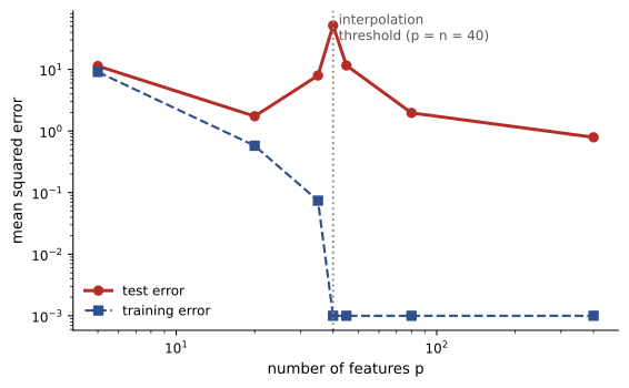
One part of the explanation is the double descent curve. As the number of parameters \(p\) grows past the number of training examples \(n\), test error first rises sharply near \(p = n\) (the interpolation threshold, where the model barely fits the data and must contort itself to do so) and then falls again as \(p\) grows further, often below the classical optimum.

import numpy as np

rng = np.random.default_rng(13)
n_train, n_test, d = 40, 1000, 5
w_true = rng.normal(size=d)
def data(n):
    X = rng.normal(size=(n, d))
    return X, X @ w_true + rng.normal(0, 0.5, n)
Xtr, ytr = data(n_train)
Xte, yte = data(n_test)

W = rng.normal(size=(d, 400)) / np.sqrt(d)               # fixed random first layer
feats = lambda X, p: np.maximum(X @ W[:, :p], 0)          # ReLU random features
print("features p   train MSE   test MSE")
for p in [5, 20, 35, 40, 45, 80, 400]:
    w = np.linalg.pinv(feats(Xtr, p)) @ ytr               # least squares, or minimum norm if p > n
    tr = np.mean((feats(Xtr, p) @ w - ytr) ** 2)
    te = np.mean((feats(Xte, p) @ w - yte) ** 2)
    print(f"{p:>10} {tr:11.3f} {te:10.3f}")

features p   train MSE   test MSE
         5       9.088     11.338
        20       0.575      1.737
        35       0.073      7.964
        40       0.000     51.630
        45       0.000     11.592
        80       0.000      1.967
       400       0.000      0.790

Beyond the threshold there are many interpolating solutions, and the minimum-norm one (Lesson 2), which gradient descent finds implicitly, becomes smoother as more features are added, so test error falls. The current understanding combines several ideas: implicit regularization by the optimizer, the inductive biases of architectures (such as convolution and attention) that favour natural solutions, and measures of complexity based on norms and flatness of the solution rather than parameter counts. It remains an active research area.