
AI-210 · Lesson 5 of 12 · 32 min
Automatic differentiation and numerical precision
Lesson 4 derived gradients by hand and implemented backpropagation for a small network. No one derives the gradients of a model with billions of parameters by hand: frameworks such as PyTorch and JAX compute them automatically from the code that computes the model. This lesson explains how automatic differentiation works, in its forward and reverse modes, why reverse mode is the right choice for training, and what it costs in memory. It then turns to the arithmetic underneath: floating-point formats, the 16-bit and 8-bit formats used to train and run large models, and the techniques, from the log-sum-exp trick to loss scaling, that keep calculations from overflowing, underflowing or losing precision.
Three ways to compute derivatives
- Symbolic differentiation manipulates formulas, as a computer algebra system does. It gives exact expressions but they can grow enormously, and it cannot easily handle programs with loops and branches.
- Numerical differentiation uses finite differences, \(f^{\prime}(x) \approx [f(x + h) - f(x - h)]/2h\). It is simple and invaluable for checking (Lesson 4), but needs one or two function evaluations per input variable and suffers from rounding error when \(h\) is small and truncation error when \(h\) is large.
- Automatic differentiation (AD) applies the chain rule to the elementary operations a program actually executes. It is exact to rounding error, handles arbitrary code, and is efficient.
Forward mode
Forward-mode AD carries, alongside every value, its derivative with respect to one chosen input. Each elementary operation updates both: for a product, \((uv)^{\prime} = u^{\prime}v + uv^{\prime}\); for a sine, \((\sin u)^{\prime} = \cos u \cdot u^{\prime}\). An elegant implementation uses dual numbers \(a + b\varepsilon\) with \(\varepsilon^{2} = 0\): evaluating a function on \(x + 1\varepsilon\) gives \(f(x) + f^{\prime}(x)\varepsilon\).
import math

class Dual:
    """A number a + b*eps with eps**2 = 0: b carries the derivative."""
    def __init__(self, val, der=0.0):
        self.val, self.der = val, der
    def __add__(self, o):
        o = o if isinstance(o, Dual) else Dual(o)
        return Dual(self.val + o.val, self.der + o.der)
    __radd__ = __add__
    def __mul__(self, o):
        o = o if isinstance(o, Dual) else Dual(o)
        return Dual(self.val * o.val, self.der * o.val + self.val * o.der)
    __rmul__ = __mul__

def sin(x):
    return Dual(math.sin(x.val), math.cos(x.val) * x.der)

def f(x):
    return 3 * x * x + sin(x) * x + 2

x = Dual(1.5, 1.0)                      # seed: dx/dx = 1
y = f(x)
exact = 6 * 1.5 + math.cos(1.5) * 1.5 + math.sin(1.5)
print(f"f(1.5) = {y.val:.6f}, f′(1.5) by forward mode = {y.der:.6f}, by hand = {exact:.6f}")f(1.5) = 10.246242, f′(1.5) by forward mode = 10.103601, by hand = 10.103601
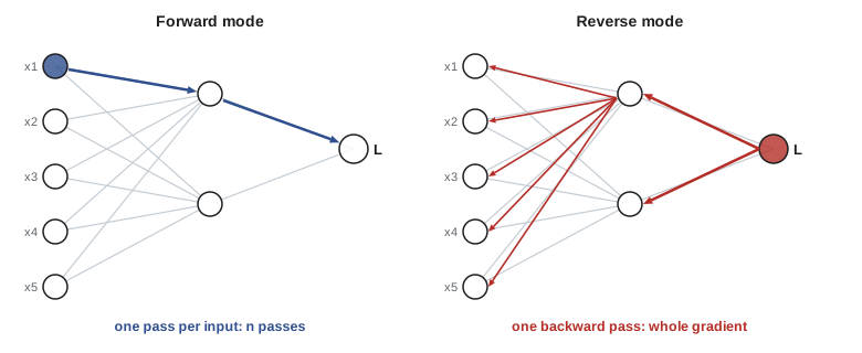
One forward pass gives the derivative of every output with respect to one input, a column of the Jacobian. For a function \(f: \mathbb{R}^{n} \to \mathbb{R}^{m}\), the full Jacobian therefore takes \(n\) forward passes. That is efficient when there are few inputs and many outputs, but training a network is the opposite case: one output (the loss) and millions or billions of inputs (the parameters).
Reverse mode
Reverse-mode AD, of which backpropagation is the special case for neural networks, works the other way. A forward pass computes the values and records the computation graph, the sequence of operations and their inputs. A backward pass then starts from the output with \(\partial L/\partial L = 1\) and visits the operations in reverse order, passing each node's adjoint \(\bar{v} = \partial L/\partial v\) back to its inputs multiplied by the local derivative:
One backward pass gives the derivative of one output with respect to every input, a row of the Jacobian, at a cost of a small constant multiple (typically two to four times) of the forward computation, regardless of the number of inputs. For a scalar loss, that is the whole gradient.
import math

class Var:
    """A scalar that records how it was computed, for reverse-mode differentiation."""
    def __init__(self, val, parents=()):
        self.val, self.parents, self.grad = val, parents, 0.0
    def __add__(self, o):
        o = o if isinstance(o, Var) else Var(o)
        return Var(self.val + o.val, [(self, 1.0), (o, 1.0)])
    def __mul__(self, o):
        o = o if isinstance(o, Var) else Var(o)
        return Var(self.val * o.val, [(self, o.val), (o, self.val)])
    def tanh(self):
        t = math.tanh(self.val)
        return Var(t, [(self, 1 - t * t)])
    def backward(self):
        order, seen = [], set()
        def visit(v):                       # topological order of the graph
            if id(v) not in seen:
                seen.add(id(v))
                for p, _ in v.parents:
                    visit(p)
                order.append(v)
        visit(self)
        self.grad = 1.0
        for v in reversed(order):           # sweep from output to inputs
            for p, local in v.parents:
                p.grad += v.grad * local

# One neuron: y = tanh(w1*x1 + w2*x2 + b), loss = y*y
x1, x2 = Var(0.5), Var(-1.5)
w1, w2, b = Var(2.0), Var(0.7), Var(0.1)
y = (w1 * x1 + w2 * x2 + b).tanh()
loss = y * y
loss.backward()
print(f"loss = {loss.val:.6f}")
print(f"dloss/dw1 = {w1.grad:.6f}, dloss/dw2 = {w2.grad:.6f}, dloss/db = {b.grad:.6f}")

h = 1e-6                                     # check one gradient numerically
f = lambda w: math.tanh(w * 0.5 + 0.7 * -1.5 + 0.1) ** 2
print(f"numerical dloss/dw1 = {(f(2.0 + h) - f(2.0 - h)) / (2 * h):.6f}")loss = 0.002496 dloss/dw1 = 0.049834, dloss/dw2 = -0.149501, dloss/db = 0.099667 numerical dloss/dw1 = 0.049834
This small class works like the autograd engines of deep learning frameworks, which do the same with tensors instead of scalars and with hand-written local derivatives for hundreds of operations. Note the += in the backward sweep: when a value is used in several places, its adjoint accumulates contributions from every use, which is the multivariable chain rule.
Worked problem
Choosing the mode
Compare the number of passes forward-mode and reverse-mode AD need for (a) the gradient of a loss with respect to 10⁹ parameters, (b) the Jacobian of a function from 3 inputs to 1,000 outputs.
Show solution
- (a) Forward mode: one pass per input, \(10^{9}\) passes. Reverse mode: one backward pass (plus the forward pass).
- (b) Forward mode: 3 passes. Reverse mode: one backward pass per output, 1,000 passes.
Answer: Reverse mode wins overwhelmingly for training (many inputs, one output); forward mode wins for functions with few inputs and many outputs, such as sensitivities of a simulation to a few design parameters. Frameworks offer both, and combine them for Hessian-vector products.
The memory cost of reverse mode
Reverse mode must keep the intermediate values of the forward pass (the activations) until the backward pass uses them. For a deep network trained on large batches, activations can need more memory than the parameters themselves. Activation checkpointing (rematerialization) stores only some activations and recomputes the rest during the backward pass, trading roughly one extra forward pass for a large memory saving; storing every \(\sqrt{L}\)-th layer of an \(L\)-layer network reduces activation memory from \(O(L)\) to \(O(\sqrt{L})\).
Worked problem
Activation memory
A transformer has 48 layers. Each layer stores about 34 activations of size batch × sequence × hidden for the backward pass, with batch 8, sequence 4,096, hidden size 4,096, in 16-bit values (2 bytes). Estimate the activation memory, and the saving from checkpointing every layer's input only.
Show solution
- Per stored tensor: \(8 \times 4{,}096 \times 4{,}096 \times 2 = 268\) MB.
- Per layer: \(34 \times 268 = 9.1\) GB; all layers: \(48 \times 9.1 = 438\) GB.
- Checkpointing only each layer's input: \(48 \times 268\) MB \(= 12.9\) GB, plus one layer's full activations (9.1 GB) during recomputation: about 22 GB.
Answer: About 440 GB without checkpointing, far more than one accelerator's memory, and about 22 GB with it, at the cost of recomputing each layer's forward pass. (The factor of 34 is a rough figure for a standard layer; real values depend on the architecture and implementation.) Memory, not arithmetic, often limits training.
Floating-point numbers
Computers represent real numbers in floating point: a sign, an exponent and a mantissa (significand), like scientific notation in base 2. The IEEE 754 standard defines the common formats. Two properties of each format matter most:
- Range, set by the exponent bits: the largest and smallest representable magnitudes. Values beyond the largest overflow to infinity; values below the smallest normal number lose precision and eventually underflow to zero.
- Precision, set by the mantissa bits: machine epsilon \(\varepsilon\), the gap between 1 and the next representable number. Relative rounding error is at most \(\varepsilon/2\).
import numpy as np

for t in [np.float16, np.float32, np.float64]:
    info = np.finfo(t)
    print(f"{t.__name__:>8}: bits {info.bits:>2}, max {info.max:9.3e}, smallest normal {info.tiny:9.3e}, "
          f"eps {info.eps:9.3e}")

with np.errstate(over="ignore"):
    big = np.float16(70000.0)                # beyond the float16 range
print("float16: 70000 ->", big, "| 1 + 0.0004 ->", np.float16(1.0) + np.float16(0.0004))

vals = np.full(10_000, 0.1)
s16 = np.float16(0)
for v in vals.astype(np.float16):            # naive running sum in half precision
    s16 = s16 + v
print("Sum of 10,000 x 0.1: float16 running sum", s16, "| float32", np.sum(vals.astype(np.float32)),
"| exact 1000")float16: bits 16, max 6.550e+04, smallest normal 6.104e-05, eps 9.766e-04 float32: bits 32, max 3.403e+38, smallest normal 1.175e-38, eps 1.192e-07 float64: bits 64, max 1.798e+308, smallest normal 2.225e-308, eps 2.220e-16 float16: 70000 -> inf | 1 + 0.0004 -> 1.0 Sum of 10,000 x 0.1: float16 running sum 256.0 | float32 1000.0001 | exact 1000
The float16 running sum stops at 256: once the total is that large, adding 0.1 is smaller than half the gap between adjacent float16 numbers (0.25 at 256), so each addition rounds back to the same value. This is absorption, and it is why accumulations are done in higher precision even when the inputs are 16-bit. Matrix-multiply hardware on accelerators multiplies 16-bit or 8-bit inputs but accumulates in 32 bits for the same reason.
Formats for machine learning
| Format | Exponent bits | Mantissa bits | Approximate range | Digits of precision | Typical use |
|---|---|---|---|---|---|
| float32 (FP32) | 8 | 23 | 10⁻³⁸ to 10³⁸ | ~7 | Master weights, accumulation |
| float16 (FP16) | 5 | 10 | 6 × 10⁻⁵ to 65,504 | ~3 | Training with loss scaling; inference |
| bfloat16 (BF16) | 8 | 7 | same as FP32 | ~2–3 | Standard for training large models |
| FP8 (E4M3 / E5M2) | 4 / 5 | 3 / 2 | about ±448 / ±57,344 | ~1 | Training and inference on recent accelerators |
Bfloat16 ("brain floating point", introduced by Google) keeps float32's 8-bit exponent and so its range, sacrificing precision. Neural network training tolerates low precision in individual values but is badly hurt by overflow and underflow, so bfloat16 usually trains without the special care float16 needs.
import numpy as np

def to_bfloat16(x):
    """Emulate bfloat16 by keeping the top 16 bits of a float32 (round to nearest even)."""
    b = np.asarray(x, dtype=np.float32).view(np.uint32)
    b = (b + 0x7FFF + ((b >> 16) & 1)) & 0xFFFF0000
    return b.view(np.float32)

for v in [1e-8, 3.14159265, 70000.0, 1.001]:
    with np.errstate(over="ignore"):
        f16 = np.float16(v)
    bf = to_bfloat16(v)
print(f"{v:>12g}: float16 {float(f16):>12.6g} bfloat16 {float(bf):>12.6g}") 1e-08: float16 0 bfloat16 1.00117e-08
3.14159: float16 3.14062 bfloat16 3.14062
70000: float16 inf bfloat16 70144
1.001: float16 1.00098 bfloat16 1Float16 underflows 10⁻⁸ to zero and overflows 70,000 to infinity, while bfloat16 represents both, but bfloat16 cannot distinguish 1.001 from 1. Choosing a format is choosing which of these failures you can live with.
Numerically stable formulas
Many formulas that are correct mathematically fail in floating point. The standard fixes are worth knowing by heart:
- Softmax and log-sum-exp: \(e^{1000}\) overflows. Subtracting the maximum, \(\log\sum_{i} e^{z_{i}} = m + \log\sum_{i} e^{z_{i} - m}\) with \(m = \max_{i} z_{i}\), gives the same answer with every exponent at most 1.
- Cross-entropy from logits: compute \(\log p_{c} = z_{c} - \text{logsumexp}(\mathbf{z})\) directly instead of taking the log of a softmax that may have underflowed to zero. Frameworks provide fused functions for exactly this reason.
- Catastrophic cancellation: subtracting nearly equal numbers loses relative precision. Computing a variance as \(E[x^{2}] - E[x]^{2}\) fails when the mean is large compared with the spread; Welford's method or subtracting the mean first avoids it.
- Small arguments: \(\log(1 + x)\) and \(e^{x} - 1\) lose precision for tiny \(x\); use log1p and expm1.
import numpy as np

z = np.array([1000.0, 999.0, 995.0])           # large logits, common late in training

with np.errstate(over="ignore", invalid="ignore"):
    naive = np.exp(z) / np.sum(np.exp(z))
print("Naive softmax:", naive)

m = z.max()
stable = np.exp(z - m) / np.sum(np.exp(z - m)) # subtract the max first
print("Stable softmax:", np.round(stable, 6))

logsumexp = m + np.log(np.sum(np.exp(z - m)))
print("log-sum-exp:", round(logsumexp, 6), "| cross-entropy for class 0:", round(logsumexp - z[0], 6))Naive softmax: [nan nan nan] Stable softmax: [0.727475 0.267623 0.004902] log-sum-exp: 1000.318175 | cross-entropy for class 0: 0.318175
Worked problem
Cancellation in a variance
Server inlet temperatures recorded in kelvin have values near 297.15 K with a spread of 0.01 K. Explain why computing the variance as mean(x²) − mean(x)² in float32 fails.
Show solution
- \(E[x^{2}] \approx 297.15^{2} = 88{,}298\) and the variance is about \(10^{-4}\).
- Float32 carries about 7 significant digits, so \(E[x^{2}]\) is known only to about \(88{,}298 \times 10^{-7} \approx 0.009\).
- The variance (0.0001) is smaller than the rounding error of the two terms being subtracted: the result is noise, possibly negative.
Answer: The subtraction cancels all the meaningful digits. Subtracting the mean before squaring (or using Welford's online algorithm) computes the variance accurately, because the squared deviations are small numbers known to full relative precision.
Mixed-precision training
Large models are trained in mixed precision: the forward and backward passes run in 16-bit (bfloat16 or float16) or even 8-bit formats on the accelerator's fast matrix units, while a 32-bit master copy of the weights receives the updates and sums are accumulated in 32 bits. With float16, small gradients can underflow to zero, so the loss is multiplied by a large scale factor before the backward pass and the gradients divided by it afterwards (loss scaling), with the factor adjusted automatically when overflows are detected. With bfloat16, loss scaling is usually unnecessary. FP8 training adds per-tensor or per-block scale factors so that each tensor uses the narrow range well. These techniques roughly double to quadruple training throughput and halve memory, and they are why the numerical details in this lesson are not academic.
Common mistakes
MistakeUsing finite differences to train models.
InsteadUse automatic differentiation; keep finite differences for checking gradients.
MistakeAssuming reverse mode is free in memory.
InsteadIt stores activations; use checkpointing when memory runs out.
MistakeAccumulating sums in 16-bit precision.
InsteadAccumulate in 32 bits even when inputs are 16-bit.
MistakeComputing softmax or log-probabilities naively.
InsteadSubtract the maximum and use log-sum-exp or fused cross-entropy functions.
MistakeComputing variance as E[x²] − E[x]².
InsteadSubtract the mean first or use Welford's algorithm.
Summary and key terms
- Automatic differentiation applies the chain rule to executed operations, exactly and efficiently.
- Forward mode gives one Jacobian column per pass; reverse mode one row per pass.
- Reverse mode (backpropagation) computes a scalar loss's full gradient in one backward pass, but stores activations.
- Floating-point formats trade range (exponent) against precision (mantissa).
- Bfloat16 keeps float32's range with less precision; float16 needs loss scaling; FP8 needs scale factors.
- Stable formulas (log-sum-exp, fused cross-entropy, centred variance, log1p) avoid overflow and cancellation.
- Mixed precision trains fast in low precision while keeping 32-bit master weights and accumulation.
- Automatic differentiation
- Computing exact derivatives by applying the chain rule to a program's operations.
- Forward mode
- AD that propagates derivatives with values from inputs to outputs.
- Reverse mode
- AD that propagates adjoints from outputs back to inputs.
- Adjoint
- The derivative of the final output with respect to an intermediate value.
- Dual number
- A number a + bε with ε² = 0, used for forward-mode AD.
- Activation checkpointing
- Recomputing some activations in the backward pass to save memory.
- Machine epsilon
- The gap between 1 and the next representable floating-point number.
- Bfloat16
- A 16-bit format with float32's exponent range and 7 mantissa bits.
- Log-sum-exp trick
- Subtracting the maximum before exponentiating to avoid overflow.
- Loss scaling
- Multiplying the loss to keep small gradients from underflowing in float16.
Practice problems
Work each problem on paper first, then reveal the answer to check.
Use dual numbers to find the derivative of x² at x = 3.
Show answer
(3 + ε)² = 9 + 6ε, so the derivative is 6.
Passes needed by forward mode for a gradient with 1,000 inputs?
Show answer
1,000.
Why does the backward pass use += for adjoints?
Show answer
A value used in several places receives contributions from each use.
What does activation checkpointing trade?
Show answer
Extra recomputation for less memory.
Largest finite float16 value?
Show answer
65,504.
Machine epsilon of float32?
Show answer
About 1.19 × 10⁻⁷.
Why does bfloat16 rarely need loss scaling?
Show answer
It has float32's exponent range, so small gradients do not underflow.
Compute log-sum-exp of (100, 100).
Show answer
100 + log 2 ≈ 100.693.
Why use log1p(x) for tiny x?
Show answer
1 + x rounds to 1, losing x; log1p computes it accurately.
Where are matrix products accumulated in mixed-precision training?
Show answer
In 32-bit precision.
Lesson quiz · 5 questions
Score 60% or more to complete this lesson.
Create a free account to save your progress, take quizzes and earn a certificate.