Vectors, matrices and decompositions

Machine learning is written in the language of linear algebra. A data point is a vector of features; a data set is a matrix with one row per example; a neural network layer is a matrix that transforms one vector into another; a word, an image or a user is represented as an embedding, a vector whose geometry captures meaning. Training adjusts matrices, and many of the most useful techniques, from principal component analysis to the low-rank adapters used to fine-tune large language models, are applications of matrix decompositions.

This course gathers the mathematics that machine learning uses most: linear algebra, matrix calculus, probability, information theory, optimization and learning theory, starting with linear algebra in this lesson. It assumes first courses in linear algebra, calculus and statistics, and focuses on the ideas as machine learning applies them. Each lesson includes short NumPy programs (the tools from AI-110) so that every idea can be computed and checked.

Vectors

A vector \(\mathbf{x} \in \mathbb{R}^n\) is an ordered list of \(n\) real numbers. In machine learning it usually represents one example: a house described by its area, age and number of rooms; a 28 × 28 image flattened into 784 pixel values; or a word represented by a learned embedding of a few hundred to a few thousand dimensions. Geometrically, a vector is a point, or an arrow from the origin, in \(n\)-dimensional space.

Dot products, norms and angles

The dot product of two vectors is the sum of the products of their components:

The Euclidean length, or \(\ell_2\) norm, is \(\|\mathbf{x}\|_2 = \sqrt{\mathbf{x}^\top\mathbf{x}}\). Other norms appear too: the \(\ell_1\) norm \(\|\mathbf{x}\|_1 = \sum |x_i|\), which encourages sparse solutions when used as a penalty, and the \(\ell_\infty\) norm, the largest absolute component. The dot product also measures the angle \(\theta\) between vectors:

This cosine similarity is the standard way to compare embeddings: it is 1 for vectors pointing the same way, 0 for perpendicular (orthogonal) vectors and −1 for opposite ones, regardless of their lengths. Search engines, recommendation systems and retrieval-augmented language models all find "similar" items by searching for vectors with high cosine similarity.

import numpy as np

# Toy 4-dimensional "embeddings" of three words
king  = np.array([0.8, 0.6, 0.1, 0.9])
queen = np.array([0.7, 0.7, 0.2, 0.8])
apple = np.array([0.1, 0.2, 0.9, 0.1])

def cosine(a, b):
    return a @ b / (np.linalg.norm(a) * np.linalg.norm(b))

print(f"|king| = {np.linalg.norm(king):.3f}")
print(f"cos(king, queen) = {cosine(king, queen):.3f}")
print(f"cos(king, apple) = {cosine(king, apple):.3f}")

|king| = 1.349
cos(king, queen) = 0.990
cos(king, apple) = 0.302

Matrices as linear maps

A matrix \(\mathbf{A} \in \mathbb{R}^{m \times n}\) is a rectangular array of numbers, and multiplying it by a vector, \(\mathbf{y} = \mathbf{A}\mathbf{x}\), maps a vector in \(\mathbb{R}^n\) to one in \(\mathbb{R}^m\). Every linear map can be written this way: rotations, scalings, reflections, projections and their combinations. Each output component is the dot product of a row of \(\mathbf{A}\) with \(\mathbf{x}\); equivalently, \(\mathbf{A}\mathbf{x}\) is a weighted sum of the columns of \(\mathbf{A}\), with weights given by \(\mathbf{x}\).

In a data matrix \(\mathbf{X} \in \mathbb{R}^{N \times d}\), each of the \(N\) rows is an example and each of the \(d\) columns is a feature. A linear model predicts \(\hat{\mathbf{y}} = \mathbf{X}\mathbf{w}\) for all examples at once, and a neural network layer computes \(\mathbf{H} = \sigma(\mathbf{X}\mathbf{W} + \mathbf{b})\), applying a nonlinearity \(\sigma\) element by element. The product of two matrices is the composition of their maps; it is associative but not commutative: in general \(\mathbf{A}\mathbf{B} \ne \mathbf{B}\mathbf{A}\).

Some special matrices recur constantly. The identity \(\mathbf{I}\) leaves vectors unchanged. The transpose \(\mathbf{A}^\top\) swaps rows and columns, with \((\mathbf{A}\mathbf{B})^\top = \mathbf{B}^\top\mathbf{A}^\top\). A symmetric matrix equals its transpose; covariance matrices and Hessians are symmetric. An orthogonal matrix \(\mathbf{Q}\) has orthonormal columns, so \(\mathbf{Q}^\top\mathbf{Q} = \mathbf{I}\): it rotates or reflects without changing lengths. A diagonal matrix scales each coordinate separately.

Rank, inverses and linear systems

The rank of a matrix is the number of linearly independent columns (equivalently rows): the dimension of the space its outputs can reach. An \(n \times n\) matrix of rank \(n\) is invertible: there is a matrix \(\mathbf{A}^{-1}\) with \(\mathbf{A}^{-1}\mathbf{A} = \mathbf{I}\), and the system \(\mathbf{A}\mathbf{x} = \mathbf{b}\) has exactly one solution. A matrix is invertible if and only if its determinant is non-zero. In numerical work, systems are solved with factorizations (np.linalg.solve) rather than by forming the inverse, which is slower and less accurate.

Eigenvalues and eigenvectors

An eigenvector of a square matrix \(\mathbf{A}\) is a non-zero vector whose direction the matrix does not change: it only scales it, by the eigenvalue \(\lambda\):

Eigenvalues are the roots of the characteristic equation \(\det(\mathbf{A} - \lambda\mathbf{I}) = 0\). Symmetric matrices have a particularly clean structure, given by the spectral theorem: all their eigenvalues are real, and their eigenvectors can be chosen orthonormal. A symmetric matrix can therefore be written \(\mathbf{A} = \mathbf{Q}\boldsymbol{\Lambda}\mathbf{Q}^\top\), where the columns of \(\mathbf{Q}\) are eigenvectors and \(\boldsymbol{\Lambda}\) is the diagonal matrix of eigenvalues. Geometrically, it stretches space by \(\lambda_i\) along each eigenvector direction.

import numpy as np

A = np.array([[2.0, 1.0],
              [1.0, 2.0]])
vals, vecs = np.linalg.eigh(A)          # eigh: for symmetric matrices
vecs = vecs * np.sign(vecs[0])          # fix signs (they are arbitrary)
print("eigenvalues:", vals)
print("eigenvectors (columns):")
print(vecs.round(3))
v = vecs[:, 1]
print("A v =", (A @ v).round(3), " lambda v =", (vals[1] * v).round(3))

eigenvalues: [1. 3.]
eigenvectors (columns):
[[ 0.707  0.707]
 [-0.707  0.707]]
A v = [2.121 2.121]  lambda v = [2.121 2.121]

Eigenvalues appear all over machine learning. The eigenvalues of a covariance matrix measure how much the data varies in each direction (the basis of PCA, below). The eigenvalues of a loss function's Hessian describe its curvature, which controls how fast gradient descent converges (Lesson 11). A symmetric matrix whose eigenvalues are all positive is positive definite: \(\mathbf{x}^\top\mathbf{A}\mathbf{x} > 0\) for every non-zero \(\mathbf{x}\). Covariance matrices are always positive semidefinite (eigenvalues ≥ 0).

The singular value decomposition

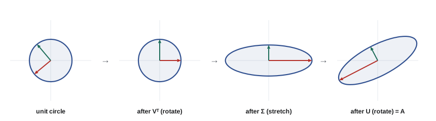
Eigendecomposition needs a square (and ideally symmetric) matrix. The singular value decomposition (SVD) works for any matrix, and it is arguably the most useful factorization in data science. Every \(m \times n\) matrix can be written

where \(\mathbf{U}\) (\(m \times m\)) and \(\mathbf{V}\) (\(n \times n\)) are orthogonal and \(\boldsymbol{\Sigma}\) is diagonal with non-negative singular values \(\sigma_1 \ge \sigma_2 \ge \dots \ge 0\). Geometrically, any linear map is a rotation (\(\mathbf{V}^\top\)), a scaling along the axes (\(\boldsymbol{\Sigma}\)) and another rotation (\(\mathbf{U}\)). The number of non-zero singular values is the rank. The singular values of \(\mathbf{A}\) are the square roots of the eigenvalues of \(\mathbf{A}^\top\mathbf{A}\).

Low-rank approximation

Keeping only the \(k\) largest singular values and their vectors gives \(\mathbf{A}_k = \mathbf{U}_k\boldsymbol{\Sigma}_k\mathbf{V}_k^\top\). By the Eckart–Young theorem, this is the best possible rank-\(k\) approximation of \(\mathbf{A}\), and its error in the Frobenius norm (the square root of the sum of all squared entries) is exactly the square root of the sum of the discarded squared singular values:

import numpy as np

rng = np.random.default_rng(0)
# A 6 x 5 matrix that is nearly rank 2, plus a little noise
U = rng.normal(size=(6, 2)); V = rng.normal(size=(2, 5))
M = U @ V + 0.05 * rng.normal(size=(6, 5))

s = np.linalg.svd(M, compute_uv=False)
print("singular values:", s.round(3))
Uf, sf, Vt = np.linalg.svd(M, full_matrices=False)
M2 = Uf[:, :2] @ np.diag(sf[:2]) @ Vt[:2]          # best rank-2 approximation
err = np.linalg.norm(M - M2)                        # Frobenius norm of the error
print(f"rank-2 error {err:.4f} = sqrt(sum of the other s^2) {np.sqrt((sf[2:]**2).sum()):.4f}")
print(f"relative error {err / np.linalg.norm(M):.4f}")

singular values: [5.054 2.148 0.116 0.079 0.024]
rank-2 error 0.1424 = sqrt(sum of the other s^2) 0.1424
relative error 0.0259

The singular values drop sharply after the second, revealing that the matrix is essentially rank 2 plus noise, and the rank-2 approximation captures it to within about 2.6%. Real data matrices (user-by-item ratings, word co-occurrence counts, images) often behave like this, which is why low-rank methods compress them so well and why recommendation systems based on matrix factorization work.

Principal component analysis

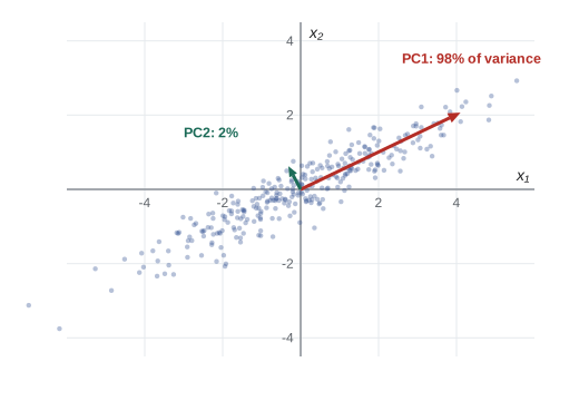
Principal component analysis (PCA) finds the directions in which data varies most. For a data matrix \(\mathbf{X}\) whose columns have been centred (mean subtracted), the covariance matrix is \(\mathbf{C} = \mathbf{X}^\top\mathbf{X}/(N - 1)\). Its eigenvectors are the principal directions, and its eigenvalues are the variances along them. In practice PCA is computed from the SVD of the centred data, \(\mathbf{X} = \mathbf{U}\boldsymbol{\Sigma}\mathbf{V}^\top\): the rows of \(\mathbf{V}^\top\) are the principal directions, and the variance along direction \(i\) is \(\sigma_i^2/(N - 1)\). The fraction of total variance explained by component \(i\) is \(\sigma_i^2/\sum_j \sigma_j^2\).

Projecting onto the first \(k\) principal components, \(\mathbf{Z} = \mathbf{X}\mathbf{V}_k\), reduces each example from \(d\) numbers to \(k\) while keeping as much variance as possible. PCA is used for visualization (projecting to two dimensions), compression, noise reduction and as a preprocessing step for other models.

import numpy as np

rng = np.random.default_rng(1)
# 500 points in 3-D that mostly vary along one direction
t = rng.normal(size=500)
X = np.column_stack([2 * t, 1 * t, 0.5 * t]) + 0.3 * rng.normal(size=(500, 3))

Xc = X - X.mean(axis=0)                      # subtract the mean of each column
U, s, Vt = np.linalg.svd(Xc, full_matrices=False)
explained = s**2 / (s**2).sum()
pc1 = Vt[0] * np.sign(Vt[0, 0])              # fix the arbitrary sign
print("explained variance ratio:", explained.round(3))
print("first principal direction:", pc1.round(3))
Z = Xc @ pc1                                 # project onto 1 component
print("projected shape:", Z.shape)

explained variance ratio: [0.96  0.022 0.018]
first principal direction: [0.87  0.442 0.219]
projected shape: (500,)

The first principal component explains 96% of the variance, and its direction (0.87, 0.44, 0.22) is close to the normalized generating direction (2, 1, 0.5)/2.29 = (0.87, 0.44, 0.22). One number per point now describes almost all of the structure in three.

How this course is organized

The course moves from linear algebra through calculus and probability to learning:

• Lessons 2 and 3 continue with linear algebra: least squares and projections, then high-dimensional geometry, embeddings and kernels.
• Lessons 4 and 5 cover matrix calculus and backpropagation, then automatic differentiation and numerical precision.
• Lessons 6 to 8 cover probability for learning, the multivariate Gaussian and Gaussian processes, and generalization theory.
• Lesson 9 covers information theory and Lesson 10 the linear algebra of deep learning.
• Lesson 11 covers convexity and optimization, and Lesson 12 builds logistic regression and a neural network from first principles.