Convexity and optimization basics

Every machine learning model is trained by solving an optimization problem: choose parameters that minimize a loss. Whether that problem is easy or hard depends largely on one property, convexity. For convex problems, any local minimum is the global minimum, gradient descent provably finds it, and the rate at which it does so can be predicted from the curvature of the loss. Linear and logistic regression, support vector machines and ridge regression are all convex. Deep neural networks are not, yet the same tools, used with care, train them successfully, and understanding the convex case is the best guide to why.

This chapter defines convex sets and functions, shows how to test for convexity, works through gradient descent on a quadratic to show how the learning rate and the condition number govern convergence, introduces Newton's method, and solves constrained problems with Lagrange multipliers. It closes with what changes for the non-convex losses of deep learning, a bridge to AI-310.

Convex sets and functions

A set is convex if the straight line between any two of its points stays inside it. Balls, half-spaces, boxes and the set of probability distributions are convex; a ring or a crescent is not.

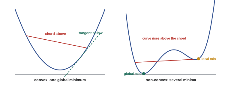
A function \(f\) is convex if its graph lies on or below every chord: for any two points and any \(t \in [0, 1]\),

Intuitively, a convex function is bowl-shaped: it never curves downward. Two equivalent tests are easier to apply when the function is differentiable:

• First-order: the function lies above all its tangents, \(f(\mathbf{y}) \ge f(\mathbf{x}) + \nabla f(\mathbf{x})^\top(\mathbf{y} - \mathbf{x})\).
• Second-order: the Hessian is positive semidefinite everywhere (for one variable, \(f\prime\prime(x) \ge 0\)). If it is positive definite everywhere, the function is strictly convex and has at most one minimizer.

Why convexity matters

The first-order condition has a powerful consequence: if \(\nabla f(\mathbf{x}^*) = 0\) at some point, then \(f(\mathbf{y}) \ge f(\mathbf{x}^*)\) for every \(\mathbf{y}\). For a convex function, every stationary point is a global minimum, and there are no local minima to get stuck in. Convexity is also preserved by useful operations, which makes it easy to recognize: non-negative weighted sums of convex functions are convex; the composition of a convex function with a linear map is convex; and the maximum of convex functions is convex.

Common convex functions in machine learning include: squared error \(\|\mathbf{X}\mathbf{w} - \mathbf{y}\|^2\); any norm, such as \(\|\mathbf{w}\|_1\) or \(\|\mathbf{w}\|_2^2\); the logistic loss \(\log(1 + e^{-y\,\mathbf{w}^\top\mathbf{x}})\); the hinge loss \(\max(0, 1 - y\,\mathbf{w}^\top\mathbf{x})\) of support vector machines; the log-sum-exp function behind softmax cross-entropy; and the negative log-likelihood of any exponential-family model with linear parameters. So regularized linear regression, logistic regression and SVMs are all convex problems with a unique global optimum.

Gradient descent on a quadratic

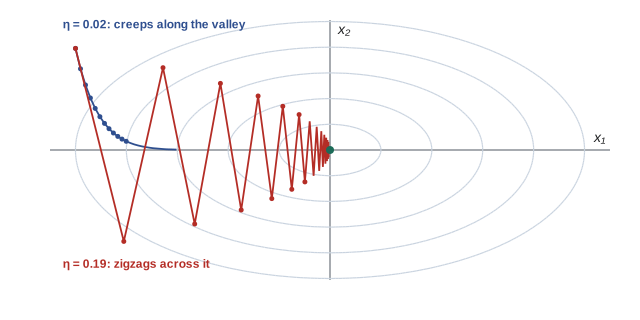
Gradient descent repeatedly steps against the gradient, \(\mathbf{x}_{k+1} = \mathbf{x}_k - \eta\nabla f(\mathbf{x}_k)\). A quadratic is the right model problem: near any minimum, a smooth function looks like one, with the Hessian supplying the curvature. Take \(f(\mathbf{x}) = \tfrac12\mathbf{x}^\top\mathbf{A}\mathbf{x}\) with \(\mathbf{A}\) symmetric positive definite, eigenvalues \(\lambda_{\min}\) to \(\lambda_{\max}\), and minimum at the origin. The gradient is \(\mathbf{A}\mathbf{x}\), so each step multiplies \(\mathbf{x}\) by \(\mathbf{I} - \eta\mathbf{A}\). Along each eigenvector the error is multiplied by \(1 - \eta\lambda_i\) per step. Two conclusions follow:

• Stability: the iteration converges only if \(|1 - \eta\lambda_i| < 1\) for all \(i\), which requires \(\eta < 2/\lambda_{\max}\). A learning rate above this diverges, however small it is compared with the other directions.
• Speed: the slowest direction is the one with the smallest curvature, which shrinks by \(1 - \eta\lambda_{\min}\) per step. The best fixed step, \(\eta = 2/(\lambda_{\min} + \lambda_{\max})\), gives a convergence factor of \((\kappa - 1)/(\kappa + 1)\) per step, where \(\kappa = \lambda_{\max}/\lambda_{\min}\) is the condition number.

An ill-conditioned problem (large \(\kappa\)), a long narrow valley, forces a small step to stay stable in the steep direction, so progress along the shallow direction is painfully slow, and the iterates zigzag across the valley.

import numpy as np

A = np.diag([1.0, 10.0])               # f(x) = 0.5 x^T A x, minimum at the origin
f = lambda x: 0.5 * x @ A @ x
x0 = np.array([10.0, 1.0])

for lr in (0.05, 0.15, 0.19, 0.21):
    x = x0.copy()
    for _ in range(100):
        x = x - lr * (A @ x)           # gradient of f is A x
    print(f"learning rate {lr:.2f}: f after 100 steps = {f(x):.3e}")

learning rate 0.05: f after 100 steps = 1.753e-03
learning rate 0.15: f after 100 steps = 3.826e-13
learning rate 0.19: f after 100 steps = 3.528e-09
learning rate 0.21: f after 100 steps = 9.495e+08

Practical remedies for ill-conditioning include standardizing input features (which can dramatically reduce \(\kappa\) for linear models), momentum, which accumulates velocity along consistent directions and damps oscillation, and adaptive methods such as Adam, which scale each parameter's step by an estimate of its gradient magnitude. AI-310 develops these in detail.

Newton's method

Gradient descent uses only the slope. Newton's method also uses the curvature: it fits the quadratic approximation from Lesson 4 at the current point and jumps to its minimum:

On a quadratic it reaches the exact minimum in one step, whatever the condition number, because multiplying by \(\mathbf{H}^{-1}\) undoes the uneven curvature. Near the minimum of a smooth function it converges quadratically: the number of correct digits roughly doubles each step. Its drawback is cost: forming and solving with the Hessian takes \(O(n^2)\) memory and roughly \(O(n^3)\) time for \(n\) parameters, which is impossible for a model with millions of weights. Quasi-Newton methods such as L-BFGS build a cheap approximation to \(\mathbf{H}^{-1}\) from recent gradients and work well for medium-sized convex problems; deep learning relies on first-order methods.

Ridge regression: a convex problem solved two ways

Ridge regression minimizes \(\|\mathbf{X}\mathbf{w} - \mathbf{y}\|^2 + \lambda\|\mathbf{w}\|^2\). Its Hessian, \(2(\mathbf{X}^\top\mathbf{X} + \lambda\mathbf{I})\), is positive definite for any \(\lambda > 0\), so the problem is strictly convex with a unique solution, \(\mathbf{w}^* = (\mathbf{X}^\top\mathbf{X} + \lambda\mathbf{I})^{-1}\mathbf{X}^\top\mathbf{y}\). Regularization also improves conditioning: adding \(\lambda\) to every eigenvalue raises the smallest one most in relative terms.

import numpy as np

rng = np.random.default_rng(5)
X = rng.normal(size=(40, 5)); y = X @ rng.normal(size=5) + 0.5 * rng.normal(size=40)
lam = 2.0

w_closed = np.linalg.solve(X.T @ X + lam * np.eye(5), X.T @ y)    # ridge, closed form

H = 2 * (X.T @ X + lam * np.eye(5))         # Hessian of ||Xw - y||^2 + lam ||w||^2
eig = np.linalg.eigvalsh(H)
print(f"Hessian eigenvalues from {eig.min():.1f} to {eig.max():.1f}: convex, condition number {eig.max() / eig.min():.1f}")

w = np.zeros(5); lr = 1.0 / eig.max()       # a safe step size
for step in range(300):
    w -= lr * (2 * X.T @ (X @ w - y) + 2 * lam * w)
print("gradient descent matches closed form:", np.allclose(w, w_closed, atol=1e-6))
print("weights:", w_closed.round(3))

Hessian eigenvalues from 49.6 to 116.0: convex, condition number 2.3
gradient descent matches closed form: True
weights: [-0.618 -2.021 -0.674 -0.066  1.025]

Constrained optimization and Lagrange multipliers

Many problems have constraints: probabilities must sum to one, a budget limits spending, a model's weights must stay within a norm ball. For an equality constraint \(g(\mathbf{x}) = 0\), the method of Lagrange multipliers says that at a constrained optimum the gradient of the objective is parallel to the gradient of the constraint, \(\nabla f = \lambda\nabla g\). In practice, form the Lagrangian \(\mathcal{L}(\mathbf{x}, \lambda) = f(\mathbf{x}) - \lambda g(\mathbf{x})\) and set all its partial derivatives to zero.

Inequality constraints, \(h(\mathbf{x}) \le 0\), are handled by the Karush–Kuhn–Tucker (KKT) conditions, which add the requirement that each multiplier is non-negative and is zero unless its constraint is active (tight). Support vector machines are derived this way: only the training points whose constraints are active, the support vectors, determine the solution. Convex problems with convex constraints keep the guarantee that a local optimum is global, and specialized solvers handle them reliably.

Beyond convexity: deep learning

Lesson 8 discusses why non-convex, over-parameterized models can still generalize, and Lesson 12 trains one from scratch.

The loss of a neural network, as a function of its weights, is not convex. It has symmetries (swapping two hidden units gives an identical network), many saddle points and, in principle, local minima. Yet gradient-based training works remarkably well. Several observations, partly theoretical and partly empirical, explain why:

• In very high dimensions, most stationary points are saddle points rather than local minima, and the noise in stochastic gradient descent helps escape them.
• Large, overparameterized networks tend to have many good minima connected by low-loss paths, so most reasonable starting points lead somewhere good.
• Careful initialization, normalization layers, residual connections and adaptive optimizers keep the local landscape reasonably well conditioned.
• The quadratic analysis still applies locally: near a minimum the Hessian sets the stable learning rate, and learning-rate warm-up and schedules (AI-310) manage the changing curvature during training.

Convex analysis remains the foundation. It provides the guarantees for linear models, the intuition for step sizes and conditioning, and the vocabulary in which the behaviour of deep networks is studied.