Linear systems, least squares and projections

Lesson 1 described matrices as linear maps and decomposed them with eigenvalues and the SVD. This lesson asks the question behind most of classical machine learning: given data \(\mathbf{X}\) and targets \(\mathbf{y}\), which weights \(\mathbf{w}\) make \(\mathbf{X}\mathbf{w}\) as close as possible to \(\mathbf{y}\)? The answer, least squares, has a beautiful geometric meaning as a projection, and understanding it explains when a regression is well posed, why some fits are numerically unstable, what "leverage" means, and how regularization picks one answer when infinitely many fit perfectly, which is the normal situation for modern over-parameterized models.

Linear systems and rank

A linear system \(\mathbf{A}\mathbf{x} = \mathbf{b}\) with \(\mathbf{A}\) of size \(m \times n\) has three possible outcomes:

• Exactly one solution, when \(\mathbf{A}\) is square and invertible (full rank).
• No exact solution, the usual case when there are more equations than unknowns (\(m > n\)), as in fitting a model to more data points than parameters: the system is overdetermined.
• Infinitely many solutions, when there are more unknowns than independent equations (\(n > m\)): the system is underdetermined.

The rank of \(\mathbf{A}\) is the number of linearly independent columns (equivalently rows): the dimension of its column space, the set of all vectors \(\mathbf{A}\mathbf{x}\) can produce. The null space is the set of \(\mathbf{x}\) with \(\mathbf{A}\mathbf{x} = \mathbf{0}\); by the rank–nullity theorem its dimension is \(n - \text{rank}(\mathbf{A})\). A design matrix with a redundant column, such as a feature duplicated in different units, is rank deficient: its null space contains directions along which the weights can change without changing the predictions, so the weights are not identifiable.

Least squares

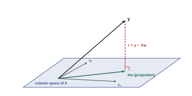
When \(\mathbf{y}\) is not in the column space of \(\mathbf{X}\), we choose \(\mathbf{w}\) to minimize the squared error \(\|\mathbf{X}\mathbf{w} - \mathbf{y}\|^{2}\). Lesson 4 derives the solution by setting the gradient to zero; here is the geometric view. The vector \(\mathbf{X}\mathbf{w}\) ranges over the column space of \(\mathbf{X}\), a flat subspace. The closest point of that subspace to \(\mathbf{y}\) is its orthogonal projection, reached when the residual \(\mathbf{r} = \mathbf{y} - \mathbf{X}\mathbf{w}\) is perpendicular to every column of \(\mathbf{X}\):

These are the normal equations ("normal" meaning perpendicular). If \(\mathbf{X}\) has full column rank, \(\mathbf{X}^{T}\mathbf{X}\) is invertible and \(\mathbf{w} = (\mathbf{X}^{T}\mathbf{X})^{-1}\mathbf{X}^{T}\mathbf{y}\).

import numpy as np

rng = np.random.default_rng(0)
n = 50
area = rng.uniform(50, 250, n)                 # floor area, m^2
age = rng.uniform(0, 60, n)                    # years
price = 40 + 2.1 * area - 0.8 * age + rng.normal(0, 15, n)   # thousands of dollars

X = np.column_stack([np.ones(n), area, age])   # design matrix with an intercept column
print("Shape of X:", X.shape, "| rank:", np.linalg.matrix_rank(X))

w, residual_ss, rank, sv = np.linalg.lstsq(X, price, rcond=None)
print("Least-squares weights:", np.round(w, 3))
r = price - X @ w
print("Residuals orthogonal to every column of X:", np.allclose(X.T @ r, 0, atol=1e-6))

X_bad = np.column_stack([X, 2 * area])        # a column that duplicates information
print("Rank with a redundant column:", np.linalg.matrix_rank(X_bad), "of", X_bad.shape[1])

Shape of X: (50, 3) | rank: 3
Least-squares weights: [48.39   2.063 -0.89 ]
Residuals orthogonal to every column of X: True
Rank with a redundant column: 3 of 4

The weights recover the coefficients used to generate the data (about 2.1 per square metre and −0.8 per year) up to noise, and the residual is orthogonal to the intercept, area and age columns, exactly as the geometry predicts. Orthogonality to the intercept column means the residuals sum to zero.

The projection matrix and leverage

The fitted values are \(\hat{\mathbf{y}} = \mathbf{X}\mathbf{w} = \mathbf{P}\mathbf{y}\), where

is the projection matrix, often called the hat matrix because it puts the hat on \(\mathbf{y}\). It is symmetric and idempotent (\(\mathbf{P}^{2} = \mathbf{P}\): projecting twice changes nothing), and its trace equals the number of parameters. Its diagonal entries \(P_{ii}\), the leverages, measure how much each observation pulls the fit toward itself. Points far from the others in feature space have high leverage: they can swing the fitted line, and a single error in such a point does disproportionate damage.

import numpy as np

rng = np.random.default_rng(1)
x = np.sort(rng.uniform(0, 10, 8))
x[-1] = 30.0                                   # one point far from the rest
X = np.column_stack([np.ones_like(x), x])
y = 3 + 0.5 * x + rng.normal(0, 0.5, x.size)

P = X @ np.linalg.inv(X.T @ X) @ X.T          # projection ("hat") matrix
print("P symmetric:", np.allclose(P, P.T), "| P idempotent (P @ P = P):", np.allclose(P @ P, P))
print("Trace of P (number of parameters):", round(np.trace(P), 6))
print("Leverage of each point:", np.round(np.diag(P), 3))
y_hat = P @ y
print("Fitted values equal X w:", np.allclose(y_hat, X @ np.linalg.lstsq(X, y, rcond=None)[0]))

P symmetric: True | P idempotent (P @ P = P): True
Trace of P (number of parameters): 2.0
Leverage of each point: [0.203 0.169 0.154 0.152 0.141 0.125 0.128 0.928]
Fitted values equal X w: True

The isolated point at \(x = 30\) has leverage 0.93: the fitted line passes almost through it whatever its \(y\) value. Because the leverages sum to the number of parameters (here 2), their average is \(p/n\), and a common rule flags points with leverage above two or three times that average for inspection.

Conditioning: when the answer is fragile

Even when \(\mathbf{X}\) has full rank, the least-squares problem can be numerically fragile. The condition number of a matrix, the ratio of its largest to smallest singular value (Lesson 1), \(\kappa(\mathbf{X}) = \sigma_{max}/\sigma_{min}\), measures how much relative errors in the data can be amplified in the solution: roughly, you can lose \(\log_{10}\kappa\) digits of accuracy. Forming the normal equations squares the condition number, \(\kappa(\mathbf{X}^{T}\mathbf{X}) = \kappa(\mathbf{X})^{2}\), which is why numerical libraries solve least squares with the QR decomposition or the SVD instead.

import numpy as np

x = np.linspace(0, 1, 40)
y = np.sin(2 * np.pi * x)
for degree in [3, 8, 14]:
    V = np.vander(x, degree + 1, increasing=True)        # columns 1, x, x^2, ...
    w_qr = np.linalg.lstsq(V, y, rcond=None)[0]           # SVD-based solver
    w_ne = np.linalg.solve(V.T @ V, V.T @ y)              # normal equations
    err_qr = np.linalg.norm(V @ w_qr - y)
    err_ne = np.linalg.norm(V @ w_ne - y)
    print(f"degree {degree:>2}: cond(V) = {np.linalg.cond(V):9.2e}, cond(VtV) = {np.linalg.cond(V.T @ V):9.2e}, "
          f"residual lstsq {err_qr:.2e}, normal eq. {err_ne:.2e}")

degree  3: cond(V) =  1.16e+02, cond(VtV) =  1.35e+04, residual lstsq 4.60e-01, normal eq. 4.60e-01
degree  8: cond(V) =  6.16e+05, cond(VtV) =  3.80e+11, residual lstsq 1.13e-03, normal eq. 1.13e-03
degree 14: cond(V) =  2.46e+10, cond(VtV) =  5.90e+17, residual lstsq 4.41e-09, normal eq. 5.85e-07

Polynomial features \(1, x, x^{2}, \ldots\) on \([0, 1]\) become nearly parallel as the degree rises, and the condition number grows enormously. At degree 14, \(\kappa(\mathbf{V}^{T}\mathbf{V})\) is around \(10^{17}\), beyond what double precision (about 16 significant digits) can represent, and the normal-equation residual is a hundred times worse than the SVD solution. The cures are to use a stable solver, to standardize features (AI-110, Lesson 6), to use better-conditioned bases such as orthogonal polynomials, or to regularize.

Underdetermined systems and the minimum-norm solution

Modern machine learning models often have far more parameters than training examples, so many weight vectors fit the training data exactly. Which one is chosen matters, because they behave differently on new data. The pseudo-inverse \(\mathbf{A}^{+}\), computed from the SVD by inverting the nonzero singular values, gives the solution of smallest Euclidean norm:

Every other solution is \(\mathbf{x}^{+}\) plus a vector from the null space, and is longer. Ridge regression, which adds a penalty \(\lambda\|\mathbf{x}\|^{2}\), approaches the minimum-norm solution as \(\lambda \to 0\).

import numpy as np

rng = np.random.default_rng(2)
A = rng.normal(size=(3, 6))            # 3 equations, 6 unknowns: infinitely many solutions
b = np.array([1.0, -2.0, 0.5])

x_min = np.linalg.pinv(A) @ b          # minimum-norm solution
print("A x = b:", np.allclose(A @ x_min, b), "| norm of x:", round(np.linalg.norm(x_min), 4))

null_basis = np.linalg.svd(A)[2][3:]  # rows spanning the null space of A
x_other = x_min + null_basis.T @ np.array([1.0, -0.5, 2.0])
print("Another solution also works:", np.allclose(A @ x_other, b), "| its norm:", round(np.linalg.norm(x_other), 4))

for lam in [1.0, 0.01, 1e-6]:
    x_ridge = A.T @ np.linalg.solve(A @ A.T + lam * np.eye(3), b)
    print(f"ridge lambda = {lam:g}: distance to minimum-norm solution {np.linalg.norm(x_ridge - x_min):.2e}")

A x = b: True | norm of x: 1.8168
Another solution also works: True | its norm: 2.9241
ridge lambda = 1: distance to minimum-norm solution 7.28e-01
ridge lambda = 0.01: distance to minimum-norm solution 1.22e-02
ridge lambda = 1e-06: distance to minimum-norm solution 1.23e-06

This has a surprising consequence. Gradient descent started from zero weights on a least-squares problem never moves in null-space directions (the gradient \(\mathbf{A}^{T}(\mathbf{A}\mathbf{x} - \mathbf{b})\) always lies in the row space of \(\mathbf{A}\)), so it converges to the minimum-norm solution without any explicit regularization. This implicit regularization by the optimizer is part of why heavily over-parameterized models can still generalize, a topic of active research (Lesson 8 and AI-310).

Orthogonality as a tool

Orthogonal matrices (\(\mathbf{Q}^{T}\mathbf{Q} = \mathbf{I}\)) preserve lengths and angles and have condition number 1, so computations with them never amplify errors. The QR decomposition \(\mathbf{X} = \mathbf{Q}\mathbf{R}\), with \(\mathbf{Q}\) having orthonormal columns and \(\mathbf{R}\) upper triangular, turns least squares into the well-conditioned triangular system \(\mathbf{R}\mathbf{w} = \mathbf{Q}^{T}\mathbf{y}\). Gram–Schmidt orthogonalization, which builds \(\mathbf{Q}\) column by column, is the classic way to understand QR; Householder reflections are the stable way to compute it. Orthogonality also appears in deep learning, where orthogonal weight initialization and orthogonality constraints help keep signals from exploding or vanishing as they pass through many layers.