
AERO-499 · Lesson 6 of 12 · 27 min
Analysis and simulation
The sizing loop rests on a handful of assumed numbers: a zero-lift drag coefficient of 0.030, an Oswald efficiency of 0.80, a drive efficiency of 0.75, a battery that delivers its energy with 5 per cent loss, and a centre of gravity that falls where the layout drawing puts it. Between weeks 12 and 16 the team checks each of these with analyses of higher fidelity, before the preliminary design review. The aim is not to replace the sizing loop with a more complicated one, but to find out whether its assumptions hold, and if not, by how much the design must change. This lesson follows three of those analyses: aerodynamics and performance, the battery through a lesson, and longitudinal stability.
Models and their fidelity
Tomasz Wierzbicki, who leads computational fluid dynamics at Borealis Aerospace, gives the team a rule he applies to his own group: use the simplest model that can answer the question, check it with a model one level higher, and validate both against something real. For drag, the levels run from a single coefficient taken from similar aircraft, through a component build-up, to a CFD solution of the whole aircraft, to a wind tunnel or flight test. Each level costs about ten times more effort than the one below. A capstone team can afford the build-up for everything, CFD for a few questions where the build-up is weak, and comparison with published data for validation.
Every model also needs verification, which is not the same as validation. Verification asks whether the code solves the equations correctly: the battery simulation must conserve energy, the drag build-up must reproduce a hand calculation, the power curve must reach its minimum where theory says it should. Validation asks whether the equations describe the real aircraft. Teams often do the first and call it the second.
Drag build-up
Owen builds up the zero-lift drag from the parts of the aircraft, each with a skin friction coefficient for its Reynolds number, a form factor for its thickness and an interference factor where it meets another part, as in the aircraft design course. Fixed undercarriage, the cooling inlets and outlets for the motor and battery, the canopy and the small items such as antennas and the pitot tube are added from data for light aircraft.
| Component | Drag area, m² | Share |
|---|---|---|
| Wing | 0.130 | 31 % |
| Fuselage and canopy | 0.098 | 23 % |
| Horizontal and vertical tail | 0.048 | 11 % |
| Fixed landing gear with fairings | 0.070 | 17 % |
| Cooling inlets and outlets | 0.028 | 7 % |
| Propeller and spinner interference, small items | 0.046 | 11 % |
| Total | 0.420 | CD0 = 0.030 on 14.0 m² |
The total confirms the 0.030 assumed in sizing, but the breakdown is more useful than the total. The fixed undercarriage is 17 per cent of the drag, more than the tail. Retractable gear would save most of it but adds 15 to 20 kg, cost and a failure mode that students would have to learn, and the school does not want it in a primary trainer. The cooling drag of 7 per cent is the item unique to electric aircraft: the motor, inverter and battery reject only a few kilowatts of heat, far less than a piston engine, so the inlets can be small, but they must work on the ground, on a hot day, with no airflow. The team sizes them for the climb and adds an electric fan for ground running.
Tomasz runs a single RANS solution of the wing, fuselage and canopy at the cruise condition as a check. It gives a drag area for those components 6 per cent below the build-up, mainly because the build-up's interference factor for the low wing root is conservative. The team keeps the build-up value, records the CFD result as evidence that the estimate is not optimistic, and does not try to resolve the difference further: at this stage a 6 per cent difference in one part of the drag is within the uncertainty of the whole design.
Power required and the speeds that matter
# Plover E2 drag polar, power required and the speeds that matter for an electric trainer
import math
g, m, S, AR, e, CD0 = 9.81, 770.0, 14.0, 11.0, 0.80, 0.030
K = 1 / (math.pi * e * AR)
rho = 1.125                         # 900 m standard day
W = m * g
eta = 0.80 * 0.94                   # propeller x electric drive
CLmax_clean = 1.45

LDmax = 1 / (2 * math.sqrt(CD0 * K))
CL_md = math.sqrt(CD0 / K)
V_md = math.sqrt(2 * W / (rho * S * CL_md))
print(f'K = {K:.4f}, L/D max = {LDmax:.1f} at CL = {CL_md:.2f}, V = {V_md:.1f} m/s ({V_md/0.5144:.0f} knots)')
Vs = math.sqrt(2 * W / (rho * S * CLmax_clean))
print(f'clean stall speed at 900 m: {Vs:.1f} m/s TAS ({Vs/0.5144:.0f} knots)')
print(f'best glide: {LDmax:.1f} km forward per km of height, sink {V_md/LDmax:.2f} m/s')

def power(V):
    CL = 2 * W / (rho * V**2 * S)
    D = 0.5 * rho * V**2 * S * (CD0 + K * CL**2)
    return D * V / eta / 1000, CL, D

print(f'\n{"V knots":>8} {"CL":>6} {"drag N":>7} {"battery kW":>11} {"Wh per km":>10}')
best_e, best_r = None, None
for kt in range(50, 116, 5):
    V = kt * 0.5144
    P, CL, D = power(V)
    print(f'{kt:8d} {CL:6.2f} {D:7.0f} {P:11.1f} {P/(V*3.6)*1000:10.0f}')
V_min = 1.3 * Vs                     # keep at least 1.3 times the clean stall speed
for i in range(500, 1200):
    V = i / 20
    if V < V_min: continue
    P = power(V)[0]
    if best_e is None or P < best_e[1]: best_e = (V, P)
    if best_r is None or P / V < best_r[1] / best_r[0]: best_r = (V, P)
print(f'\nlowest speed considered: {V_min/0.5144:.0f} knots (1.3 Vs)')
print(f'best endurance (minimum power): {best_e[0]/0.5144:.0f} knots, {best_e[1]:.1f} kW')
print(f'best range (minimum energy per km): {best_r[0]/0.5144:.0f} knots, {best_r[1]:.1f} kW, {best_r[1]/(best_r[0]*3.6)*1000:.0f} Wh/km')
usable_eol = 59.1 * 0.90 * 0.85 * 0.95
print(f'usable energy at end of life after losses {usable_eol:.1f} kWh -> endurance at best endurance speed {usable_eol/best_e[1]*60:.0f} min')K = 0.0362, L/D max = 15.2 at CL = 0.91, V = 32.5 m/s (63 knots)
clean stall speed at 900 m: 25.7 m/s TAS (50 knots)
best glide: 15.2 km forward per km of height, sink 2.14 m/s
V knots CL drag N battery kW Wh per km
50 1.45 552 18.9 204
55 1.20 517 19.4 191
60 1.01 500 20.5 185
65 0.86 499 22.2 184
70 0.74 508 24.3 188
75 0.64 528 27.1 195
80 0.57 555 30.4 205
85 0.50 589 34.2 217
90 0.45 629 38.7 232
95 0.40 674 43.8 249
100 0.36 724 49.5 268
105 0.33 779 56.0 288
110 0.30 838 63.1 310
115 0.27 902 70.9 333
lowest speed considered: 65 knots (1.3 Vs)
best endurance (minimum power): 65 knots, 22.2 kW
best range (minimum energy per km): 65 knots, 22.2 kW, 184 Wh/km
usable energy at end of life after losses 43.0 kWh -> endurance at best endurance speed 116 minThe polar gives a maximum lift-to-drag ratio of 15.2 at 63 knots. At 80 knots, the normal cruise, the aircraft needs 30.4 kW from the battery; at 90 knots, 38.7 kW. The cost of speed is steep: the energy per kilometre rises from 184 Wh at 65 knots to 232 Wh at 90, so the extra 10 knots of the normal cruise against the speed for best range cost about 12 per cent in energy per kilometre. Both best endurance and best range fall at or below 1.3 times the clean stall speed, which is as slow as the team is willing to plan a reserve. In practice the aircraft has a single economical speed, around 65 knots, at which its endurance on the end-of-life usable energy is almost two hours.
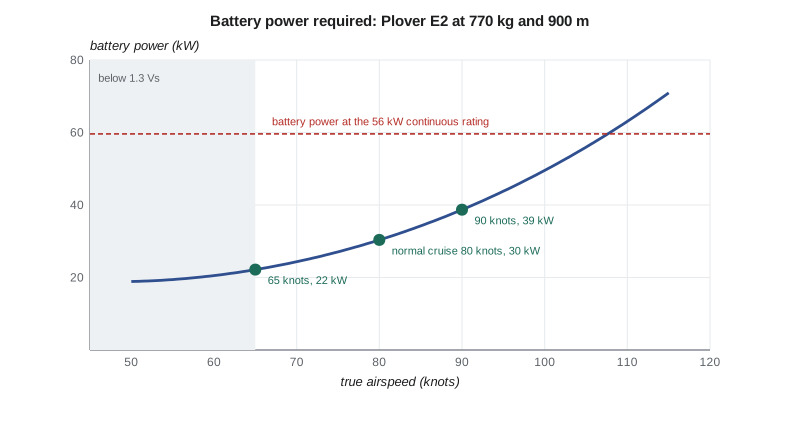
This is the source of a choice the school will have to make. If the normal cruising speed is set at 65 knots in the flight manual, the reserve required by the operating rules costs 11 kWh instead of 15, and the 4 kWh freed would lengthen the lesson by about 7 minutes, as the worked example below shows. Sam is against it. At 65 knots a trainer is slow in the circuit, uncomfortable in gusty winds and at the edge of the speed range where students should be taught; he wants the normal cruise to be a speed pilots actually use. The team keeps 80 knots for the design and records the slower cruise as an operational option the school may choose later, with the regulator's agreement.
The battery through a lesson
The sizing loop treated the battery as a store of energy with a fixed efficiency. A real battery is a voltage source whose voltage falls as it discharges and as the current rises, with an internal resistance that rises sharply when the cells are cold and as they age. Lucas builds a time-stepped model of the pack: at each 10-second step it finds the current that delivers the required power, given the open-circuit voltage at the present state of charge and the internal resistance, then updates the state of charge and the heat generated. The cell model, an open-circuit voltage curve and a resistance of 30 milliohms per cell at 20 °C, comes from the supplier's data sheet; lesson 8 describes how the team checks it on the bench.
The mission passes if the state of charge at landing after the full reserve is at least 5 per cent and the cell voltage never falls below 3.0 V, below which the cells age quickly and the motor cannot reach full power.
# Time-stepped mission simulation for the Plover E2 battery: state of charge, voltage and heat
cells_s, cells_p = 108, 30            # 108 series groups of 30 cells in parallel (two packs of 15p in parallel)
Q_cell = 5.0                          # Ah per cell, new
segments = [('taxi', 8, 4.0), ('take-off and climb', 6, 65.4), ('lesson', 34, 34.8),
            ('descent and landing', 5, 13.6), ('reserve at 80 knots', 30, 30.3)]

def ocv(soc):                         # open-circuit voltage per cell, simple fit for NMC cells
    return 3.30 + 0.85 * soc - 0.30 * (1 - soc) ** 6 + 0.05 * soc ** 8

def fly(cap_factor, r_factor, label, T0=20, soc0=0.95):
    Q = Q_cell * cells_p * cap_factor          # Ah per series group
    R = 0.030 / cells_p * r_factor            # ohm per group: cell 30 milliohm new at 20 C
    soc, t, vmin, heat, out = soc0, 0.0, 9e9, 0.0, []
    for name, minutes, kw in segments:
        for _ in range(int(minutes * 6)):      # 10 s steps
            v_oc = ocv(soc) * cells_s
            R_pack = R * cells_s
            # solve P = V I with V = v_oc - I R  ->  R I^2 - v_oc I + P = 0
            P = kw * 1000
            disc = v_oc**2 - 4 * R_pack * P
            if disc < 0: return f'{label:34s} voltage collapse during {name}'
            I = (v_oc - disc ** 0.5) / (2 * R_pack)
            V = v_oc - I * R_pack
            vmin = min(vmin, V); heat += I**2 * R_pack * 10 / 3.6e6
            soc -= I * 10 / 3600 / Q; t += 10
        out.append((name, soc))
    dT = heat * 3.6e6 / (300 * 1000)          # 300 kg of pack, 1000 J/(kg K), no cooling
    flag = 'reserve intact' if soc >= 0.05 and vmin / cells_s >= 3.0 else 'reserve NOT intact'
    return f'{label:34s} end SOC {soc*100:5.1f} %  min cell {vmin/cells_s:4.2f} V  heat {heat:4.2f} kWh  pack {T0}->{T0+dT:.0f} C  {flag}'

print(f'pack: {cells_s}s{cells_p}p, nominal {cells_s*3.65:.0f} V, {cells_s*cells_p*Q_cell*3.65/1000:.1f} kWh')
print(fly(1.00, 1.0, 'new pack, 20 C', 20))
print(fly(0.85, 1.5, 'end of life, 20 C', 20))
print(fly(0.85 * 0.88, 1.5 * 2.2, 'end of life, cold soaked to -10 C', -10))
print(fly(0.85 * 0.97, 1.5 * 1.2, 'end of life, pre-warmed to 10 C', 10))
print(fly(0.85 * 0.99, 1.5 * 1.05, 'end of life, pre-warmed to 15 C', 15))
print(fly(0.85, 1.5 * 0.85, 'end of life, hot day 35 C', 35))pack: 108s30p, nominal 394 V, 59.1 kWh new pack, 20 C end SOC 23.3 % min cell 3.36 V heat 1.06 kWh pack 20->33 C reserve intact end of life, 20 C end SOC 7.4 % min cell 3.04 V heat 1.70 kWh pack 20->40 C reserve intact end of life, cold soaked to -10 C end SOC -17.3 % min cell 1.90 V heat 4.81 kWh pack -10->48 C reserve NOT intact end of life, pre-warmed to 10 C end SOC 3.2 % min cell 2.91 V heat 2.11 kWh pack 10->35 C reserve NOT intact end of life, pre-warmed to 15 C end SOC 6.1 % min cell 3.00 V heat 1.81 kWh pack 15->37 C reserve intact end of life, hot day 35 C end SOC 8.0 % min cell 3.07 V heat 1.43 kWh pack 35->52 C reserve intact
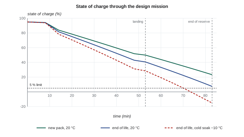
A new pack at 20 °C finishes the reserve with 23 per cent left. At end of life the margin shrinks to 7.4 per cent, and the lowest cell voltage is 3.04 V, just above the limit. The design meets R2 at 20 °C, but only just, which is what a design sized to its requirement should do.
The cold cases are the important ones for a school at St. Andrews. A pack cold soaked overnight to −10 °C has more internal resistance and less available capacity, and it fails badly: the voltage falls below the limit during the reserve and the state of charge goes negative, which in reality means the battery management system would cut power. Even a pack warmed to 10 °C fails narrowly. At 15 °C it passes with 6.1 per cent. The model is pessimistic for the cold cases, because a real pack warms itself as it discharges and its resistance falls, but the conclusion holds: in Winnipeg winters, when the airfield sits below −25 °C for days at a time, the pack must be warm at take-off. This is why R10 calls for the charger to pre-condition the battery. The team writes the operating limit into the draft flight manual: battery temperature at least 15 °C before take-off, with a cockpit display of pack temperature and a take-off inhibit below 5 °C.
The simulation also changed the sizing. The first sizing loop had no discharge loss, and the simulation showed that the end-of-life pack ran out of energy during the reserve. Adding the 5 per cent loss to the sizing loop raised the mass from 741 to 768 kg. That is the value of a higher-fidelity check: it found an error of 27 kg in the design before anything was built.
Longitudinal stability
Grace estimates the neutral point, the centre of gravity position at which the aircraft would be neutrally stable in pitch, from the wing, the tail and corrections for the fuselage and the tractor propeller, using the method of the flight mechanics course:
# Neutral point, centre of gravity range and static margin for the Plover E2
import math
S, c, AR = 14.0, 1.13, 11.0
a = 2 * math.pi * AR / (2 + math.sqrt(AR**2 + 4))       # wing lift slope per rad
St, lt, ARt, eta_t = 2.6, 4.0, 4.5, 0.90                 # horizontal tail area, arm, aspect ratio, efficiency
at = 2 * math.pi * ARt / (2 + math.sqrt(ARt**2 + 4))
VH = St * lt / (S * c)
deps = 2 * a / (math.pi * AR)                            # downwash gradient
dh_fus, dh_prop = -0.075, -0.030                         # fuselage and tractor propeller (estimates)
hn = 0.25 + eta_t * VH * (at / a) * (1 - deps) + dh_fus + dh_prop
print(f'tail volume {VH:.2f}, downwash gradient {deps:.2f}, neutral point {hn*100:.1f} % MAC')

LEMAC = 1.98                                              # m from the datum at the propeller spinner
items = {'motor, inverter, propeller': (55, 0.45), 'front battery pack': (150, 0.95),
         'airframe and systems': (225, 2.75), 'aft battery pack': (150, 3.30)}
m0 = sum(m for m, _ in items.values()); M0 = sum(m * x for m, x in items.values())
print(f'empty mass {m0} kg, empty CG {(M0/m0-LEMAC)/c*100:.1f} % MAC')
cases = {'solo student 55 kg': [(55, 2.35)], 'solo student 100 kg': [(100, 2.35)],
         'two of 90 kg': [(180, 2.35)], 'two of 90 kg and 10 kg bags': [(180, 2.35), (10, 3.05)],
         'two of 100 kg and 20 kg bags': [(200, 2.35), (20, 3.05)]}
for name, load in cases.items():
    m = m0 + sum(w for w, _ in load); M = M0 + sum(w * x for w, x in load)
    h = (M / m - LEMAC) / c
    print(f'{name:30s} mass {m:4.0f} kg  CG {h*100:5.1f} % MAC  static margin {(hn-h)*100:5.1f} %')
print('the battery does not burn off, so the CG does not move in flight')tail volume 0.66, downwash gradient 0.30, neutral point 46.6 % MAC empty mass 580 kg, empty CG 20.2 % MAC solo student 55 kg mass 635 kg CG 21.3 % MAC static margin 25.3 % solo student 100 kg mass 680 kg CG 22.1 % MAC static margin 24.5 % two of 90 kg mass 760 kg CG 23.2 % MAC static margin 23.4 % two of 90 kg and 10 kg bags mass 770 kg CG 24.1 % MAC static margin 22.5 % two of 100 kg and 20 kg bags mass 800 kg CG 25.2 % MAC static margin 21.4 % the battery does not burn off, so the CG does not move in flight
The neutral point is at 46.6 per cent of the mean chord. The centre of gravity runs from 21.3 per cent with a light solo student to 24.1 per cent with two 90 kg occupants and baggage, giving static margins between 22.5 and 25.3 per cent. The last case, two 100 kg occupants with 20 kg of baggage, exceeds the maximum take-off mass and is shown only to illustrate how little the centre of gravity moves: three per cent of the chord across every loading. The reason is the layout. The occupants sit close to the centre of gravity, the two packs balance each other, and nothing burns off in flight.
The margin is larger than a trainer needs; 10 to 15 per cent would give stable, pleasant handling with lower stick forces and less trim drag. The team has two choices: move the wing aft relative to the fuselage by about 10 cm, or keep the tail smaller. The tail size is set by the elevator power needed to flare at the forward limit with full flap, not by stability, so the team moves the wing in detailed design. Arjun notes that this small centre of gravity range is one of the real advantages of the battery aircraft: a piston trainer's centre of gravity moves with fuel burn and with the wide range of occupants and fuel loads it can carry, and its tail must be sized for that range.
Other analyses
The team also estimates the dynamic modes with the linear models of the flight mechanics course: a well-damped short period of about 3 seconds, a lightly damped phugoid of about 30 seconds, a Dutch roll of about 2.5 seconds with adequate damping, and a slightly divergent spiral mode, all typical of light trainers. The noise in the circuit at a distance of 300 m, estimated from the propeller tip speed and blade loading, is about 7 dB below the school's piston trainer, a difference residents near St. Andrews would notice. And Fatima runs the loads that feed the structure, which is the subject of the next lesson.
Worked problem
Choosing the normal cruising speed
Using the power curve, compare the energy for the 30-minute reserve at 80 knots and at 65 knots. How much longer could the lesson be if the cruise were set at 65 knots, flying the lesson at 15 per cent above 80-knot cruise power?
Show solution
- Reserve at 80 knots: \(30.4 \times 0.5 = 15.2\) kWh. At 65 knots: \(22.2 \times 0.5 = 11.1\) kWh.
- Energy freed: \(15.2 - 11.1 = 4.1\) kWh.
- Lesson power: \(1.15 \times 30.4 = 35.0\) kW.
- Extra lesson time: \(4.1/35.0 = 0.117\) h, about 7 minutes.
Answer: About 4 kWh, or 7 minutes of lesson at lesson power. Seven minutes is a modest gain for a cruise speed that pilots would rarely fly, which is why the team kept 80 knots.
Common mistakes
MistakeCalling a verified model validated.
InsteadVerify that the code solves its equations, then validate the equations against real data.
MistakeTreating the battery as an ideal energy store.
InsteadModel voltage, internal resistance, temperature and ageing over the whole mission.
MistakeReporting only the total drag.
InsteadUse the breakdown to find what is worth improving, such as gear and cooling drag.
MistakeSizing the tail for stability alone.
InsteadCheck the trim and flare cases at the forward centre of gravity, which often set the tail size.
Summary and key terms
- Analyses of higher fidelity test the sizing assumptions.
- A component drag build-up confirms a zero-lift drag coefficient of 0.030, with gear 17 per cent and cooling 7 per cent; a RANS check comes out 6 per cent lower on the wing and fuselage.
- The power curve gives a maximum lift-to-drag ratio of 15.2 at 63 knots, 30.4 kW at the 80-knot cruise and 22.2 kW at 65 knots.
- A time-stepped battery model shows the end-of-life pack meets the mission at 20 °C with 7.4 per cent left, fails after a cold soak and passes when pre-warmed to 15 °C, and that the pack heats by about 17 °C in a mission on a hot day.
- The simulation found a 27 kg sizing error.
- The neutral point is at 46.6 per cent chord and the static margin 22.5 to 25.3 per cent across all loadings, because the centre of gravity barely moves.
- Verification
- Checking that a model solves its equations correctly.
- Validation
- Checking that the model describes the real system.
- Drag build-up
- Estimate of total drag from the drag of each component.
- Internal resistance
- Resistance inside a cell that causes voltage drop and heat.
- Neutral point
- Centre of gravity position of neutral longitudinal stability.
- Static margin
- Distance from the centre of gravity to the neutral point, as a fraction of the mean chord.
Practice problems
Work each problem on paper first, then reveal the answer to check.
Why does the team keep the drag build-up value rather than the lower CFD result?
Show answer
The difference is within the design's uncertainty, and the build-up is the conservative value.
What two limits define a mission pass in the battery model?
Show answer
State of charge at least 5 per cent after the reserve and cell voltage never below 3.0 V.
What did the battery simulation change in the sizing?
Show answer
It added a 5 per cent discharge loss, raising the mass from 741 to 768 kg.
Why does the Plover E2's centre of gravity barely move?
Show answer
Occupants sit near it, the packs balance each other, and no fuel burns off.
What sets the horizontal tail size?
Show answer
Elevator power to flare with full flap at the forward centre of gravity.
Lesson quiz · 5 questions
Score 60% or more to complete this lesson.
Create a free account to save your progress, take quizzes and earn a certificate.